


As a response to the generalized food crisis of the early 1970s, the Committee on World Food Security prompted the creation of the Global Information and Early Warning System on Food and Agriculture (GIEWS). Over the years, GIEWS has established itself as the world’s leading source of information and as a respected authority on global food production, consumption and trade. It continuously monitors the food security situation in every country of the world and alerts the world to emerging food shortages. more...
Latest from GIEWS


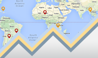
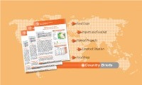
- Country Briefs updated in past 10 days:
