CHAPTER 3

ROAD DESIGN

3.1 Horizontal and Vertical Alignment

Center line alignment influences haul cost, construction cost, and environmental cost (e.g., erosion, sedimentation). During the reconnaissance phase and pre-construction survey the preliminary center line has been established on the ground. During that phase basic decisions regarding horizontal and vertical alignment have already been made and their effects on haul, construction, and environmental costs. The road design is the phase where those "field" decisions are refined, finalized and documented.

3.1.1 Horizontal Alignment Considerations

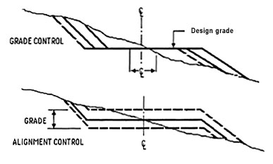
The preferred method for locating low volume roads discussed in Section 2.3, the so called non-geometric or "free alignment" method, emphasizes the importance of adjusting the road alignment to the constraints imposed by the terrain. The main difference between this and conventional road design methods is that with the former method, the laying out and designing of the centerline offset is done in the field by the road locator while substantial horizontal offsets are often required with the latter method (Figure 25).

Figure 25. Non-geometric and conventional p-line traverses.

Adjustments in horizontal alignment can help reduce the potential for generating roadway sediment. The objective in manipulating horizontal alignment is to strive to minimize roadway cuts and fills and to avoid unstable areas. When unstable or steep slopes must be traversed, adjustments in vertical alignment can minimize impacts and produce a stable road by reducing cuts and fills. The route can also be positioned on more stable ground such as ridgetops or benches. Short, steep pitches used to reach stable terrain must be matched with a surface treatment that will withstand excessive wear and reduce the potential for surface erosion. On level ground, adequate drainage must be provided to prevent ponding and reduce subgrade saturation. This can be accomplished by establishing a minimum grade of 2 percent and by rolling the grade.

Achieving the required objectives for alignment requires that a slightly more thoughtful preliminary survey be completed than would be done for a more conventionally designed road. There are two commonly accepted approaches for this type of survey: the grade or contour location method (used when grade is controlling), or the centerline location method (used when grades are light and alignment is controlling). Figure 26 illustrates design adjustments that can be made in the field using the non-geometric design concept discussed earlier.

Figure 26. Design adjustments.

Equipment needed for ether method may include a staff compass, two Abney levels or clinometers, fiberglass engineer's tape (30 or 50 m), a range rod, engineering field tables, notebook, maps, photos, crayons, stakes, flagging, and pencils. The gradeline or contour method establishes the location of the P-line by connecting two control points with a grade line. A crew equipped with levels or clinometers traverses this line with tangents that follow, as closely as possible, the contours of the ground. Each section is noted and staked for mass balance calculations. Centerline stakes should be set at even 25 - and 50 - meter stations when practicable and intermediate stakes set at significant breaks in topography and at other points, such as breaks where excavation goes from cut to fill, locations of culverts, or significant obstructions.

On gentle topography with slopes less than 30 percent and grade is not a controlling factor, the centerline method may be used. Controlling tangents are connected by curves established on the ground. The terrain must be gentle enough so that by rolling grades along the horizontal alignment, the vertical alignment will meet minimum requirements. In general, this method may be less practical than the gradeline method for most forested areas.

When sideslopes exceed 50 - 55 percent or when unstable slope conditions are present, it may be necessary to consider full bench construction shown in Figure 27. Excavated material in this case must be end hauled to a safe location. Normally, the goal of the road engineer is to balance earthwork so that the volume of fill equals the volume of cut plus any gain from bulking less any loss from shrinkage (Figure 28).

Road design, through its elements such as template (width, full bench/side cast), curve widening and grade affect the potential for erosion. Erosion rates are directly proportional to the total exposed area in cuts and fills. Road cuts and fills tend to increase with smooth, horizontal and vertical alignment. Conversely, short vertical and horizontal tangents tend to reduce cuts and fills. Erosion rates can be expected to be lower in the latter case. Prior to the design phase it should be clearly stated which alignment, horizontal or vertical, takes precedence. For example, if the tag line has been located at or near the permissible maximum grade, the vertical alignment will govern. Truck speeds in this case are governed by grade and not curvature. Therefore, horizontal alignment of the center line can follow the topography very closely in order to minimize earthwork. Self balancing sections would be achieved by shifting the template horizontally.

Figure 27. Full bench design

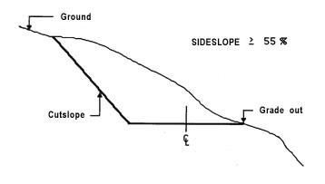
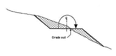
Figure 28. Self-balanced design.

3.1.2 Curve Widening

Roadway safety will be in jeopardy and the road shoulders will be impacted by off-tracking wheels if vehicle geometry and necessary curve widening are not considered properly. Continually eroding shoulders will become sedimentation source areas and will eventually weaken the road. On the other hand, over design will result in costly excessive cuts and/or fills.

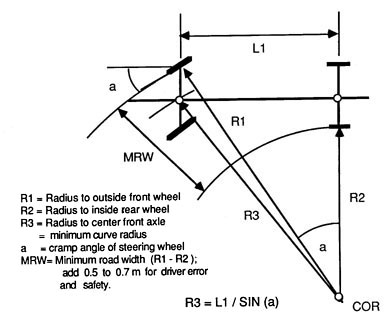
The main principle of off-tracking and hence curve widening, centers on the principle that all vehicle axles rotate about a common center. Minimum curve radius is vehicle dependent and is a function of maximum cramp angle and wheelbase length (see Figure 29).

Figure 29. Basic vehicle geometry in off-tracking.

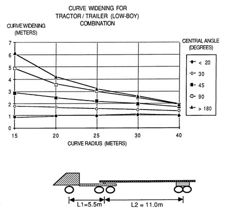
Typical vehicle dimensions are shown in Figure 30 for single trucks, truck/ trailers, log truck (pole-type), and tractor/trailer combinations. These dimensions were used to develop Figures 35 to 38 for calculating curve widening in relation to curve radius and central angle.

Several different solutions to determine curve widening requirements are in use. Most mathematical solutions and their simplified versions give the maximum curve widening required. Curve widening is a function of vehicle dimensions, curve radius, and curve length (central angle).

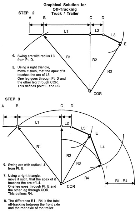
A graphical solution to the problem is provided in Figures 31 to 33. This solution can be used for single trucks, truck-trailer combinations and vehicle overhang situations. This solution provides the maximum curve widening for a given curve radius.

Figure 30. Example of truck-trailer dimensions.

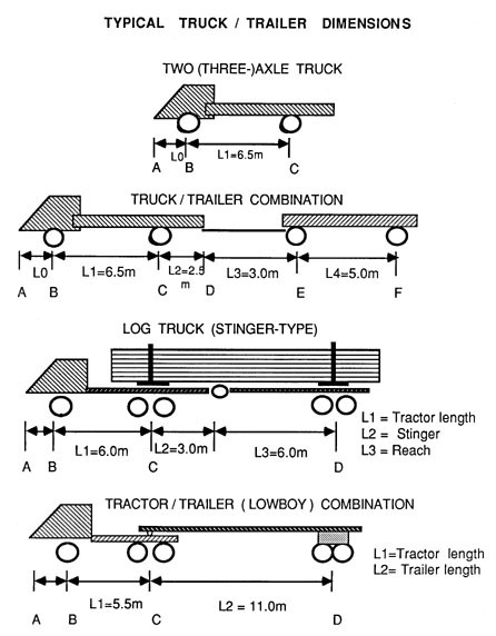
Figure 31. Sept 1. Graphical solution of widening

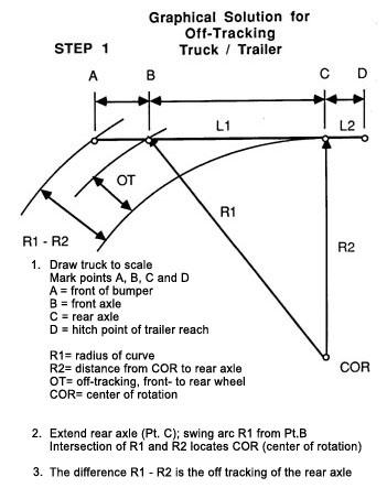
Figure 32. Steps 2 and 3. Graphical solution for curve widening.

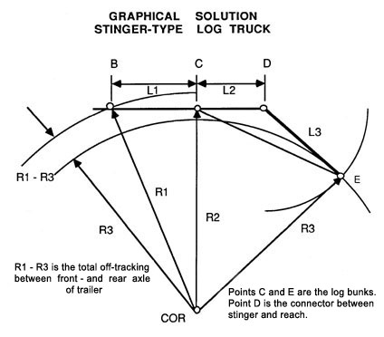
The graphical solution for a stinger type log truck is shown in Figure 33. Here, an arc with the bunk length L2 plus L3 is drawn with the center at C. The log load swivels on the bunks, C and E and forms line C - E, with the trailer reach forming line D - E.

Figure 33. Graphical solution for off-tracking of a stinger-type log truck.

Simple, empirical curve widening formulae have been proposed by numerous authors and government agencies. A common method used in North America is:

CW = 37/R For Tractor-trailer (low boy; units in meters)

CW = 18.6/R For log-truck (units in meters)

The above equations are adapted for the typical truck dimensions used in the United States and Canada. In Europe, curve widening recommendations vary from 14/R to 32/R. Curve widening recommendations in Europe are given by Kuonen (1983) and Dietz et al. (1984). Kuonen defines the curve widening requirement for a two-axle truck (wheelbase = 5.5m) as

CW = 14/R

and a truck-trailer combination where

CW = 26/R

Dietz, et. al. (1984) recommend CW = 32/R for any truck combination.

The approximation methods mentioned above are usually not satisfactory under difficult or critical terrain conditions. They typically overestimate curve widening requirements for wide curves (central angle < 45º) and under estimate them for tight curves (central angle > 50º).

Vehicle tracking simulation provides a better vehicle off-tracking solution because it considers vehicle geometry and curve elements, in particular the deflection angle (Kramer, 1982, Cain & Langdon, 1982). The following charts provide off-tracking for four common vehicle configurations--a single or two-axle truck, a truck-trailer combination, a stinger-type log-truck and a tractor-trailer (lowboy) combination. The charts are valid for the specified vehicle dimensions and are based on the following equation (Cain and Langdon, 1982):

OF = (R - (R2 - L2)1/2) * (1 - eX)

For a log-truck:

L = (L1(2) + L2(2) + L3(2))1/2

where L1-3 are defined in Figure 30.

The maximum off-tracking for a given vehicle, radius and deflection angle occurs when the vehicle leaves the curve. Since vehicles travel both directions, the required curve widening, which consists of off-tracking (OT) plus safety margin (0.5 - 0.6m), should be added to the full curve length. One half of the required curve widening should be added to the inside and one half to the outside of the curve (Figure 34).

Figure 34. Curve widening and taper lengths.

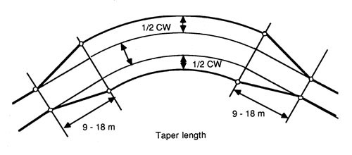
Figures 35 through 38 provide vehicle off-tracking for a given vehicle, radius, and deflection (or central angle). To this value, 0.5 to 0.6m should be added to allow for formula and driver's error, grade, and road or super elevation variations. Transition or taper length from tangent to curve vary from 9 to 18 m depending on curve radius. Recommended length of transition before and after a curve are as follows (Cain and Langdon, 1982):

Example: Standard road width is 3.0 m. Design vehicle is a stinger-type log-truck with dimensions as shown in Figure 30. Curve radius is 22m, deflection angle equals 60º.

From Figure 37 locate curve radius on the x-axis (interpolate between 20 and 25), go up to the corresponding 60º - curve (interpolate between 45º and 90º), go horizontally to the left and read the vehicle off-tracking equal to 1.8 m.

The total road width is 4.80 m (3.0 m + 1.8 m).

Depending on conditions, a safety margin of 0.5 m could be added . The current 3.0 m road width already allows for safety and driver's error of 0.30 m on either side of the vehicle wheels (truck width = 2.40 m ). Depending on the ballast depth, some additional shoulder width may be available for driver's error. Taper length would be 15 m.

Figure 35. Curve widening guide for a two or three axle truck as a function of radius and deflection angle. The truck dimensions are as shown.

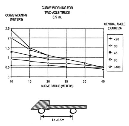
Figure 36. Curve widening guide for a truck-trailer combination as a function of radius and deflection angle. The dimensions are as shown.

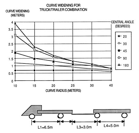
Figure 37. Curve widening guide for a log-truck as a function of radius and deflection angle. The dimensions are as shown.

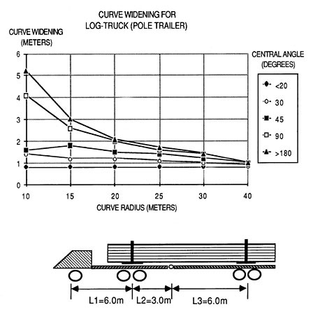
Figure 38. Curve widening guide for a tractor/trailer as a function of radius and deflection angle. The tractor-trailer dimensions are as shown.

3.1.3 Vertical Alignment

Vertical alignment is often the limiting factor in road design for most forest roads. Frequently grades or tag lines are run at or near the maximum permissible grade. Maximum grades are determined by either vehicle configuration (design/critical vehicle characteristic) or erosive conditions such as soil or precipitation patterns. Depending on road surface type, a typical logging truck can negotiate different grades. Table 16 lists maximum grades a log truck can start from. It should be noted that today's loaded trucks are traction limited and not power limited. They can start on grades up to 25 % on dry, well maintained, unpaved roads. Once in motion they can typically negotiate steeper grades.

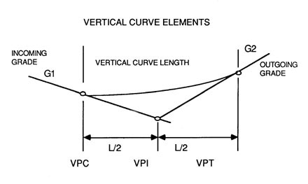
Vertical curves or grade changes, like horizontal curves, require proper consideration to minimize earthwork, cost, and erosion damage. Proper evaluation requires an analysis of vertical curve requirements based on traffic characteristics (flow and safety), vehicle geometry, and algebraic difference of intersecting grades.

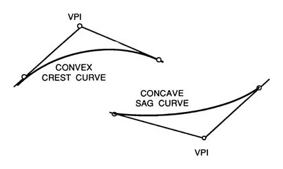
Vertical curves provide the transition between an incoming grade and an outgoing grade. For convenience in design, a parabolic curve (Figures 39 and 40) is used because the grade change is proportional to the horizontal distance. The grade change is the difference between incoming grade and outgoing grade. The shorter the vertical curve can be kept, the smaller the earthwork required.

Figure 39. Typical vertical curves (VPI = Vertical Point of Intersection).

The grade change per unit length is defined as

(G1 - G2) / L (% / meter)

or more commonly its inverse, where the grade change is expressed in horizontal distance (meters) to effect a 1% change in grade.

Table 16. Maximum grades log trucks can start on from rest (Cain, 1981).

Figure 40. Vertical curve elements (VPC = Vertical Point of Curvature; VPT = Vertical Point of Tangency).

Factors to be considered in the selection of a vertical curve are:

Stopping Sight distance S: On crest curves, S is a function of overall design speed of the road and driver's comfort. On most forest roads with design speeds from 15 km/hr to 30 km/hr, the minimum stopping sight distance is 20 and 55 meters respectively ( see Ch. 2.1.2.7 ). Kuonen (1983) provides an equation for minimal vertical curve length based on stopping distance:

Lmin = Smin2 / 800

Example: Determine the minimum vertical curve length for a crest curve that satisfies the safe stopping sight distance.

Design speed of road: 25 km/hr
Grade change (G1 - G2): 20 %

Solution: Stopping sight distance for 25 km/hr equals approximately 37 meters (from Ch. 2.1.2.7).

Lmin = (37(2) / 800) 20 = 34.2 m

Vehicle geometry: Vehicle clearance, axle spacing, front and rear overhang, freedom of vertical movement at articulation points are all factors to be considered in vertical curve design.

Passage through a sag curve requires careful evaluation of the dimensions as illustrated in Figure 41.

Figure 41. Log truck geometry and dimensions for vertical curve analysis

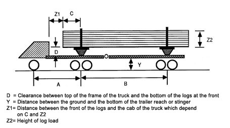
The critical dimensions of a log truck when analyzing crest vertical curves are the length of the stinger and the vertical distance between the stinger and the bottom of the logs, x. A log truck as shown in Figure 41 with dimension

could negotiate a grade change of 30% over a vertical curve length of 12 m without damage to the truck (Ohmstede, 1976).

As shown in the previous example , safety considerations typically require significantly longer, vertical curves than physical truck dimensions do. With the exception of special or critical vehicles, vertical curves can be kept very short, even for large grade changes. Road maintenance considerations are more important in such situations. Vehicle dimension considerations do become important, however, in special cases such as fords in creek crossings.

3.2 Road Prism

Proper design of the roadway prism can significantly reduce the amount of sediment and debris that enters adjacent streams. Often the basic cause of a particular mass failure can be traced to overroading or overdesign. Overroading or misplacement of roads results from a poor land management or transportation plan; overdesign results from rigidly following design criteria with respect to curvature, width, gradient, and oversteepened cuts and fills or from designing roads to higher standards than are required for their intended use. As stated previously, allowing terrain characteristics to govern road design permits more flexibility and will be especially beneficial, both environmentally and economically, where it is possible to reduce cut and fill slope heights, slope angles, and roadway widths.

3.2.1 Road Prism Stability

Stability considerations as applied to natural slopes are also valid for stability analysis of road cuts and fills. Points to consider include

- Critical height of cut slope or fill slope
- Critical piezometric level in a slope or road fill
- Critical cut slope and fill slope angle.

The most common road fill or sidecast failure mode is a translational slope failure. Translational slope failure is characterized by a planar failure surface parallel to the ground or slope. Depth to length ratio of slides are typically very small. The following slopes would fall into this category:

1. Thin, residual soil overlaying an inclined bedrock contact
2. Bedrock slopes covered with glacial till or colluvium
3. Homogeneous slopes of coarse textured, cohesionless soils (road fills)

Fill slope failure can occur in two typical modes. Shallow sloughing at the outside margins of a fill is an example of limited slope failure which contributes significantly to erosion and sedimentation but does not directly threaten the road. It is usually the result of inadequate surface protection. The other is sliding of the entire fill along a contact plane which can be the original slope surface or may include some additional soil layers. It results from lack of proper fill compaction and/or building on too steep a side slope. Another reason could be a weak soil layer which fails under the additional weight placed on it by the fill.

Slope or fill failure is caused when forces causing or promoting failure exceed forces resisting failure (cohesion, friction, etc.). The risk of failure is expressed through the factor of safety (see Figure 2):

FS = Shear strength / Shear stress

where shear strength is defined as

T = C * A + N (tan [f])

and shear stress, the force acting along the slope surface, is defined as

D = W * sin [b]

Table 17. Values of friction angles and unit weights for various soils. (from Burroughs, et. al., 1976)

The friction angle is also referred to as the angle of repose. Sand or gravel cannot be used to form a steeper slope than the frictional angle allows. In other words, the maximum fill angle of a soil cannot exceed its coefficient of friction. Typical friction angles are given in Table 17. One should note the change in soil strength from "loose" to "compact" indicating the improvement in cohesion brought about by proper soil compaction.

Cohesionless soils such as sands or gravel without fines (clay) derive their strength from frictional resistance only

T = W * cos[b] * tan[f]

while pure clays derive their shear strength from cohesion or stickiness. Shear strength or cohesive strength of clay decreases with increasing moisture making clays very moisture sensitive.

The factor of safety against sliding or failure can be expressed as:

FS = {C * A + (W * cos[b] * tan [f])} / {W * sin[b]}

In cases where the cohesive strength approaches zero (granular soils, high moisture content) the factor of safety simplifies to

FS = tan[f] / tan[b], (C = 0)

Road fills are usually built under dry conditions. Soil strength, particularly, cohesive strength is high under such conditions. If not planned or controlled, side cast fills are often built at the maximum slope angle the fill slope will stand (angle of repose). The fill slope, hence, has a factor of safety of one or just slightly larger than one. Any change in conditions, such as added weight on the fill or moisture increase, will lower the factor of safety, and the fill slope will fail. It is clear that the factor of safety must be calculated from "worst case" conditions and not from conditions present at the time of construction.

Failure can be brought about in one of two ways:

1. Translational fill failure (Figure 42) can be brought about by a build-up of a saturated zone. Frictional strength or grain-to-grain contact is reduced by a bouyancy force. Rainfall and/or ponded ditch water seeping into the fill are often responsible for this type of failure.

Figure 42. Translational or wedge failure brought about by saturated zone in fill. Ditch overflow or unprotected surfaces are often responsible.

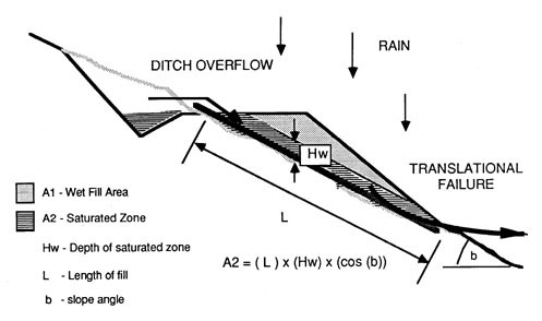
The factor of safety against a translational failure can be shown to be:

FS = {[ C * A1 + g buoy * A2] * tan[f]} / {[ g * A1 + gsat * A2] * tan[b]}

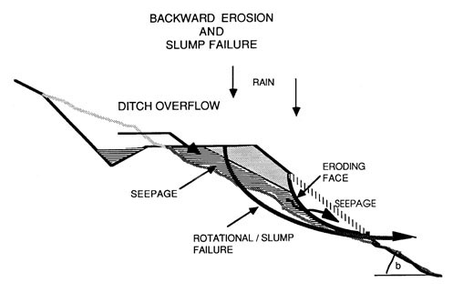
2. Rotational or Slump fill failure brought about by seepage at the toe of the fill (Figure 43). The subsequent backward erosion of unprotected fill toes will result in a vertical face or bank prone to slumping. Eventually it will trigger a complete fill failure.

Figure 43. Fill failure caused by backward erosion at the toe of the fill due to excessive seepage and an unprotected toe.

Stability analysis can help in the determination and selection of proper road prism. Fill slope angle for common earth (a mixture of fragmented rock and soil) should typically not exceed 33.6º which corresponds to a rise: run ratio of 1:1.5. Therefore, a road prism on side slopes steeper than 50 - 55% (26 - 29º) should be built as "full-benched" because of the marginal stability of the fill section. Fill sections on steep side slopes can be used, if the toe of the fill is secured through cribbing or a rock wall which allows a fill slope angle of 33.6º (1:1.5).

Practical considerations suggest that fill slope angle and ground slope angle should differ by at least 7º. Smaller angles result in so-called "sliver-fills" which are difficult to construct and erode easily.

Example:

Ground slope = 50%
Fill slope = 66.7%

Assuming zero cohesion and friction angle equals fill angle ([f] = [b])

FS = tan[f] / tan[b] = 0.667 / 0.50 = 1.33

The factor of safety is adequate. The fill slope stability becomes marginal if the same road prism (fill clone angle = 33 7º) is built on a 60% side Slope The factor of safety becomes

FS = 0.667 / 0.600 = 1.11

The factor of safety in this case would be considered marginal. Here the. difference between fill slope angle and ground slope is less than 7º, a sliver fill.

Cut slope failures in road construction typically occur as a rotational failure. It is common in these cases to assume a circular slip surface. Rotational failures can be analyzed by the method of slices, probably the most common method for analyzing this type of failure (Bishop, 1950; Burroughs, et. al.,1976).

Numerous stability charts have been developed for determining the critical height of a cut for a specific soil characterized by cohesion, friction angle, and soil density. The critical Neigh Hcrit, is the maximum height at which a slope will remain stable. They are related to a stability number, Ns, defined as

Ns = Hcrit (C/[g])

Chen and Giger (1971) and Prellwitz (1975) published slope stability charts for the design of cut and fill slopes. Cut/fill slope and height recommendations in Section 3.2.3 are based on their work.

3.2.2 Side Cast - Full Bench Road Prism

Proper road design includes the selection of the appropriate road template as well as minimal earthwork by balancing the cuts and fills as shown in Figure 44.

Figure 44. Elements of road prism geometry.

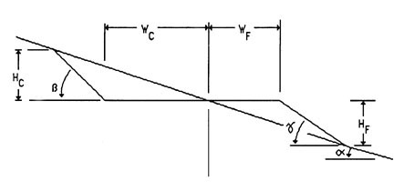
The volume of cut and fill per meter of road can be calculated by the following formula:

For earthwork calculations, the required fill equals the cut, minus any loss from shrinkage, plus any gain from swell (rock).

Fill slopes can be constructed up to a maximum slope angle of 36° to 38°. Common practice is to restrict fill slopes to 34º. This corresponds to a ratio of 1 : 1.5 (run over rise). The maximum fill slope angle is a function of the shear strength of the soil, specifically the internal angle of friction. For most material, the internal angle of friction is approximately 36° to 38°.

Compacted side cast fills which must support part of the road become more difficult to construct with increasing side slopes. Sliver fills, as described in Section 3.2.1, result from trying to construct fills on steep side slopes. For side slopes in excess of 25° to 27° (50 to 55 %), the full road width should be moved into the hillside. Excavated material can be side cast or wasted, but should not form part of the roadbed or surged for the reasons discussed in Chapter 3.2.1.

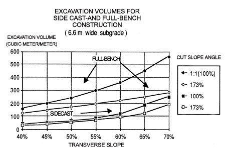
The volume of excavation required for side cast construction varies significantly with slope. On side slopes less than 25° to 30° (50 to 60%) the volume of excavation for side cast construction is considerably less than the volume of excavation for full bench construction. However, as the side slope angle approaches 75% (37°), the volume of excavation per unit length of road for side cast construction approaches that required for full bench construction. Side cast fills, however, cannot be expected to remain stable on slopes greater than 75%.

This relationship of excavation volume for side cast and full bench construction is shown in Figure 45. The subgrade width is 6.6 meter, the fill angle is 37°, and a bulking factor of 1.35 is assumed (expansion due to fragmentation or excavation of rock).

A similar graph can be reconstructed by the following equation:

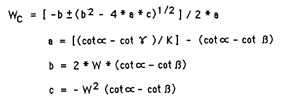
Figure 45. Required excavation volumes for side cast and full bench construction as function of side slope. Assumed subgrade width 6.6 m and bulking factor K = 1.35 (rock).

where:

W = total subgrade width

= WC + WF

K = bulking or compaction factor

(for rock, K = 1.3 - 1.4; for common earth compacted fills, K = 0.7 - 0.8. Other symbols are defined earlier in this section.)

The effect of careful template selection on overall width of disturbed area becomes more important with increasing side slope. Material side cast or "wasted" on side slopes steeper than 70 to 75% will continuously erode since the side slope angle exceeds the internal angle of friction of the material. The result will be continuous erosion and ravelling of the side cast material.

Another factor contributing to the instability of steeply sloping fills is the difficulty in revegetating bare soil surfaces. Because of the nature of the side cast material (mostly coarse textured, infertile soils) and the tendency for surface erosion on slopes greater than 70%, it is very difficult to establish a permanent protective cover. From that perspective, full bench construction combined with end haul of excavated material (removing wasted material to a safe area) will provide a significantly more stable road prism.

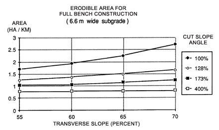
The relationship between erodible area per kilometer of road surface increases dramatically with increasing side slope where the excavated material is side cast (Figure 46). The affected area (erodible area), however, changes very little with increasing side slopes for full bench construction combined with end haul (Figure 47). The differences in affected area between the two construction methods are dramatic for side slopes exceeding 60%.

Figure 46 . Erodible area per kilometer of road for side cast construction as a function of side slope angle and cut slope angle. The values shown are calculated for a 6.6 m wide subgrade. The fill angle equals 37º.

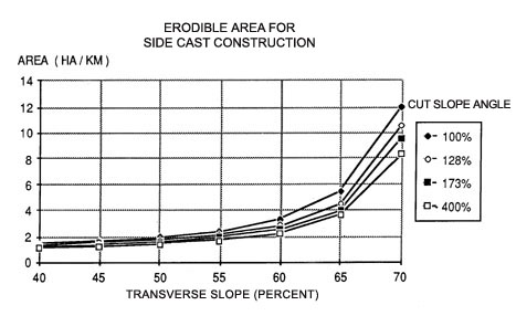
For example, the difference in affected area is over 8.8 km² per kilometer of road as the side slope angle approaches 65%. Also, as slope angle increases, the erosive power of flowing water increases exponentially. Obviously, careful consideration must be given when choosing between side cast construction and full bench construction with end haul.

Figure 47 . Erodible area per kilometer of road for full bench/end haul construction as a function of side slope angle and cut slope angle. The values shown are calculated for a 6.6 m wide subgrade.

3.2.3 Slope design

The U. S. Forest Service has developed guidelines for determining general values for maximum excavation and embankment slope ratios based on a combination of general field descriptions and the Unified Soil Classification of the material. Water table characteristics along with standard penetration and in-place density test values can further define the nature of the materials. Published information sources describing soils, geology, hydrology, and climate of the area should be carefully reviewed since certain of these reports often contain specific information relating to the engineering properties of materials in the area. These will also assist in the detailed characterization of soils, geologic, and bedrock conditions along the entire cross section of cut and/or fill area.

In general, the higher the cut or fill the more critical the need becomes for accurate investigation. The following consists of special limitations with regard to height of the cut or fill and the level of investigation required to adequately describe the entire-cross section.

0 to 15 meters (0 to 50 feet) in vertical height requires a minimum of investigation for non-critical areas The investigation would include soil classification, some hand or backhoe excavation, seismic data, and observations of nearby slopes to determine profile horizonation and relative stability.

15 to 30 meters (50 to 100 feet) in vertical height requires a more extensive investigation including all the items listed above plus test borings, either by hand auger or drill holes to identify soil horizons and the location of intermittent or seasonal water tables within the profile.

Over 30 meters (over 100 feet) in vertical height will require a slope designed by a specialist trained in soil mechanics or geological engineering. Under no circumstances should the following guides be used for slopes in excess of 30 meters in vertical height.

Special investigation may also be necessary when serious loss of property, extensive resource damage, or loss of life might result from a slope failure or when crossing areas where known instability exists or past slope failures have occurred. Soils containing excessive amounts of organic matter, swelling clays, layered schists or shales, talus, and pockets of loose water- bearing sands and silts may require special investigation as would fissured clay deposits or layered geologic strata in which subsurface conditions could not be determined for visual or seismic investigation.

The following list shows soil types and the pertinent design figures and tables for that soil:

Curves generated in Figures 48 and 49 illustrating maximum cut slope angles for coarse grained soils are organized according to five soil types:

1. Well graded material with angular granular particles; extremely dense with fines that cannot be molded by hand when moist; difficult or impossible to dig with shovel; penetration test blow court greater than 40 blows per decimeter.

2. Poorly graded material with rounded or low percentage of angular granular particles; dense and compact with fines that are difficult to mold by hand when moist; difficult to dig with shovel; penetration test approximately 30 blows per decimeter.

3. Fairly well graded material with subangular granular particles; intermediate density and compactness with fines that can be easily molded by hand when moist (Plasticity Index > 10); easy to dig with shovel; penetration test blow count approximately 20 blows per decimeter.

4. Well graded material with angular granular particles; loose to intermediate density; fines have low plasticity (Plasticity Index < 10); easy to dig with shovel; penetration test blow count less than 10 blows per decimeter.

5. Poorly graded material with rounded or low percentage of granular material; loose density; fines have low plasticity (Plasticity Index < 10); can be dug with hands; penetration count less than 5 blows per decimeter.

Curves generated in Figures 50 and 51 illustrating maximum cut slope angles for fine grained soils are organized according to five soil types based on consistency. Complete saturation with no drainage during construction is assumed making the depth to a slowly permeable underlying layer such as bedrock or unweathered residual material the single most important variable to consider. Figure 50 assumes the critical depth to be at or above the bottom of the cut; Figure 51 assumes the critical depth to be at a depth three times the depth -of excavation as measured from the bottom of the cut. Cut slope values for intermediate depths can be interpolated between the two charts:

1. Very stiff consistency; soil can be dented by strong pressure of fingers; ripping may be necessary during construction; penetration test blow count greater than 25 blows per decimeter.

2. Stiff consistency; soil can be dented by strong pressure of fingers; might be removed by digging with shovel; penetration test blow count approximately 20 blows per decimeter.

3. Firm consistency; soil can be molded by strong pressure of fingers; penetration test blow count approximately 10 blows per decimeter.

4. Soft consistency; soil can easily be molded by fingers; penetration test blow count approximately 5 blows per decimeter.

5. Very soft consistency; soil squeezes between fingers when fist is closed; penetration test blow count less than 2 blows per decimeter.

Fill slopes typically display weaker shear strengths than cut slopes since the soil has been excavated and moved from its original position. However, fill strengths can be defined with a reasonable degree of certainty, provided fills are placed with moisture and density control. The slope angle or angle of repose is a function of the internal angle of friction and cohesive strength of the soil material. Table 20 provides a recommended maximum fill slope ratio as a function of soil type, moisture content, and degree of compaction. Slopes and fills adjacent to culvert inlets may periodically become subjected to inundation when ponding occurs upstream of the inlet.

Compaction control, as discussed previously, is achieved through the manipulation of moisture and density and is defined by the standard Proctor compaction test (AASHTO 90). If no compaction control is obtained, fill slopes should be reduced by 25 percent.

Table 18. Maximum cut slope ratio for coarse grained soils. (USFS, 1973).

Table 19. Maximum cut slope ratio for bedrock excavation (USFS, 1973).

Figure 48. Maximum cut slope ratio for coarse grained soils with plastic fines (low water conditions). Each curve indicates the maximum height or the steepest slope that can be used for the given soil type. (After USFS, 1973).

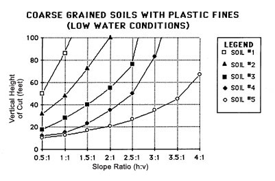
Figure 49. Maximum cut slope angle for coarse grained soils with plastic fines (high water conditions). Each curve indicates the maximum cut height or the steepest slopes that can be used for the given soil type. (After USFS, 1973).

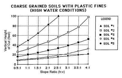
Figure 50. Maximum cut slope angle for fine grained soils with slowly permeable layer at bottom of cut. Each curve indicates the maximum vertical cut height or the steepest slope that can be used for the given soil type. (After USES 1973).

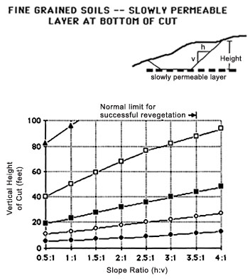
Figure 51. Maximum cut slope angle for fine grained soils with slowly permeable layer at great depth (>= 3 times height of cut) below cut. (After USES, 1973).

Table 20. Minimum fill slope ratio for compacted fills. (US Forest Service, 1973).

3.2.4 Road Prism Selection

In the planning stage (Chapter 2) basic questions such as road uses, traffic volume requirements and road standards have been decided. The road standard selected in the planning stage defines the required travel width of the road surface. The road design process uses the travel width as a departure point from which the necessary subgrade width is derived. The road design process which deals with fitting a road template into the topography uses the subgrade width for cut and fill calculations. Therefore, ditch and ballast requirements need to be defined for a given road segment in order to arrive at the proper subgrade width or template to be used.

Example: (see also Figure 52.): Travelled road width is established at 3.0 meters. Ballast material is pit-run rock. Shoulder slope of ballast is 2:1. Soil and traffic characteristics require 0.45 m layer of ballast. The ditch line is to be 0.30 m deep with slopes of 1:1 and 2:1. Fill widening of 0,6 m is added because of fill slope height.

Total subgrade width is therefore:

Figure 52. Interaction of subgrade dimension, roadwidth, ballast depth, ditch width and fill widening.

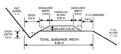
Table 21 lists various subgrade width for a 3.00 m traveled road width and different ballast depth requirements.

Table 21. Required subgrade width (exclusive fo fill widening) as a function of road width, ballast depth and ditch width. Roadwidth = 3.0 m, ditch = 0.9 m (1:1 and 2:1 slopes), shoulder-slopes 2:1.

Fill widening is another factor which modifies the subgrade or template width independent of traveled road width or ballast depth. Fill widening should be considered in cases where fills cannot be compacted with proper equipment and where no compaction control is performed. In such cases fill widening of 0.30 m are recommended where fill slope height is less than 2.00 m. Fill slope height in excess of 2.00 m should have 0,60 m of fill widening (see Figure 53). Fill slope height in excess of 6.00 m should be avoided altogether because of potential stability problems.

Cut slopes are inherently more stable than fill slopes. The road designer should try to minimize fill slope length by "pushing the alignment into the hill side in order to minimize erosion. Typically this will result in longer cut slopes and add slight to moderate cuts at the center line. The result will be a moderate fill slope (see Figure 54) with no additional fill widening required.

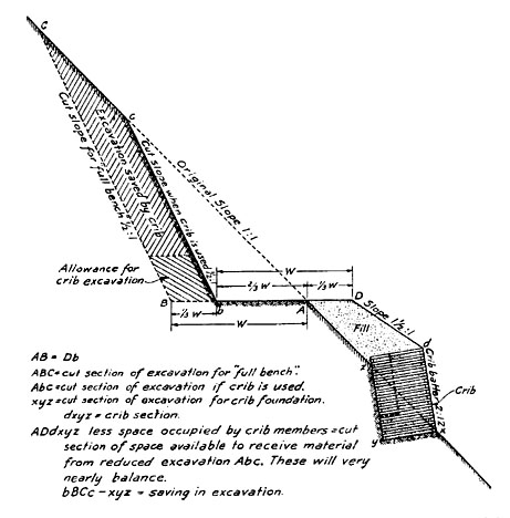
Toe walls are often a feasible alternative on steep side slopes to reduce excavation and avoid end hauling. Toe walls can be built of log cribs, gabions or large rocks (Figure 55). A proper base foundation is excavated at the toe of the fill on which the retaining wall is constructed. Approximately two-thirds of the subgrade would be projected into the hill side and one third would be supported by the fill resting on the retaining structure. The reduction in excavation material, exposed cut slope and avoided end haul is significant.

Figure 53. Fill widening added to standard subgrade width where fill height at centerline or shoulder exceeds a critical height. Especially important if sidecast construction instead of layer construction is used.

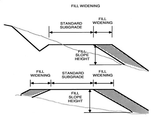
Figure 54. Template and general road alignment projected into the hill favoring light to moderate cuts at centerline in order to minimize fill slope length. Fill slopes are more succeptible to erosion and sloughing than cut slopes.

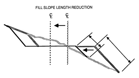
Figure 55. Illustration of the very considerable reduction in excavation made possible on a steep slope by the use of cribbing. Crib proportions shown are suitable for log construction; if crib was built of concrete or steel, shorter spreaders could be used in upper 3 m as indicated by the dashed line (Kraebel, 1936).

3.3 Road Surfacing

Properly designed road surfaces serve a dual purpose. First, they provide a durable surface on which traffic can pass smoothly and safely. If heavy all-season use is anticipated, the surface should be designed to withstand the additional wear. Second, the road surface must protect the subgrade by distributing surface loads to a unit pressure the subgrade can support, minimizing frost action, and providing good surface drainage. A crowned surface of 3 to 5 cm/m of half-width will ensure adequate movement of surface water and reduce the potential for subgrade saturation.

Improper road surfacing or ballasting affects water quality in two ways: 1) Surface material is ground up into fines that are easily eroded. It has been demonstrated that surface loss is related to traffic levels and time in addition to erosional forces. Larger gravels present in the road surface must be mechanically ground up by traffic before they can be acted upon by surface erosion processes (Armstrong, 1984).

Reid and Dunne (1984) have demonstrated the significance of traffic intensity in the mobilization of sediment in an area of the Pacific Northwest Region of the United States which receives an average annual rainfall of 3900 mm/yr (150 in/yr). The results from their study demonstrated that although road segments receiving "heavy" use accounted for only a small proportion of total road length in the basin study area (6 percent), 70 percent of the total amount of sediment generated from road surfaces could be attributed to those segments during periods of heavy use. Reid and Dunne found the sediment production for a paved and gravelled road to be 2.0 and 500 tonnes/km/year, respectively (Table 22).

Table 22. Calculated sediment yield per kilometer of road for various road types and use levels (Reid, 1981; Reid and Dunne, 1984).*

Heavy use consisted of 4 to 16, 30 tonne log-trucks per day. Temporary non-use occurred over weekends with no log-truck traffic but occassional light vehicles. Light use was restricted to light vehicles (less than 4 tonnes GVW).

A road surface in its simplest form consists of a smoothed surface, in effect the subgrade. Dirt roads would fall into this category. Obviously, dirt roads are only useful where the road is expected to receive intermittent, light use and is not affected by climate. Sediment production from dirt road surfaces is high. Significant erosion rate reductions can be achieved by applying a rock or ballast layer. Even a minimal rock surface of 5 to 10 cm effectively reduces erosion and sediment yield by a factor of 9. Kochenderfer and Helvey (1984) documented soil loss reduction from 121 down to 14 tonnes per hectare per year by applying a 7.5 cm rock surface on a dirt road.

Inadequate ballast or rock layers will not provide wheel load support appropriate for the subgrade strength except in cases where the subgrade consists of heavily consolidated materials. As a result, the ballast material is pushed into the subsoil and ruts begin to form. Ruts prevent effective transverse drainage, and fine soil particles are brought to the surface where they become available for water transport. Water is channeled in the ruts and obtains velocities sufficient for effective sediment transport. Sediment yield from rutted surfaces is about twice that of unrutted road surfaces (Burroughs et. al., 1984).

An improvement over a simple dirt road consists of a ballast layer over a subgrade, with or without a wearing course. The function of the ballast layer is to distribute the wheel load to pressures the subsoil can withstand. The wearing course provides a smooth running surface and also seals the surface to protect the subgrade from surface water infiltration. The wearing course can either be a crushed gravel layer with fines or a bitumenous layer.

Required ballast depth or thickness not only depends on subgrade strength but also on vehicle weight and traffic volume. The time or service life a road can support traffic without undue sediment delivery depends on:

- soil strength
- ballast depth
- traffic volume (number of axles)
- vehicle weight (axle load)

Surface loading from wheel pressure is transmitted through the surface to the subgrade in the form of a frustrum of a cone. Thus, the unit pressure on the subgrade decreases with increasing thickness of the pavement structure. Average unit pressure across the entire width of subgrade for any wheel load configuration can be calculated from the following formula:

A useful parameter for determining the strength of subgrade material is the California Bearing Ratio (CBR). CBR values are indices of soil strength and swelling potential. They represent the ratio of the resistance of a compacted soil to penetration by a test piston to penetration resistance of a "standard material", usually compacted, crushed rock (Atkins, 1980). The range of CBR values for natural soils is listed in Table 23 together with their suitability as subgrade material. Poorer subgrade material requires a thicker ballast layer to withstand traffic load and volume.

Factors other than CBR values must be considered when determining the thickness of the pavement structure. Subgrade compaction will depend upon construction methods used and the control of moisture during compaction. Subgrade drainage effectiveness, frost penetration and frost heave, and subgrade soil swell pressure are associated with water content in the soil and will also affect final design thickness. To counteract these factors, a thicker, heavier pavement structure should be designed.

Table 23. Engineering characteristics of soil groups for road construction (Pearce, 1960).

An alternative to the cost of a heavier pavement structure is the use of geotextile fabrics. Fabrics have been found to be an economically acceptable alternative to conventional construction practices when dealing with less than desirable soil material. The U. S. Forest Service has successfully used fabrics as filters for surface drainage, as separatory features to prevent subgrade soil contamination of base layers, and as subgrade restraining layers for weak subgrades. A useful guide for the selection and utilization of fabrics in constructing and maintaining low volume roads is presented by Steward, et al. (1977). This report discusses the current knowledge regarding the use of fabrics in road construction and contains a wealth of information regarding physical properties and costs of several brands of fabric currently marketed in the United States and abroad.

Proper thickness design of ballast layer not only helps to reduce erosion but also reduces costs by requiring only so much rock as is actually required by traffic volume (number of axles) and vehicle weight (axle weight-wheel loads). The principle of thickness design is based on the system developed by AASHO (American Association of State Highway Officials) and adapted by Barenberg et al. (1975) to soft soils. Barenberg developed a relationship between required ballast thickness and wheel or axle loads. Soil strength can be simply measured either with a cone penetrometer or vane shear device, such as a Torvane.

Thickness design for soft soil is based on the assumption of foundation shear failure where the bearing capacity of the soil is exceeded. For rapid loading, such as the passage of a wheel, the bearing capacity q is assumed to depend on cohesion only.

Based on Barenberg's work, Steward, et al. (1977) proposed a value of 2.8 to 3.3 and 5.0 to 6.0 for Nc. The significance of the bearing capacity q is as follows:

A. q = 2.8 C is the stress level on the subgrade at which very little rutting will occur under heavy traffic (more than 1000 trips of 8,160 kg axle equivalencies) without fabric.

B. q = 3.3 C is the stress level at which heavy rutting will occur under light axle loadings (less than 100 trips of 8,160 kg axle equivalencies) without fabric.

C. q = 5.0 C is the stress level at which very little rafting would be expected to occur at high traffic volumes (more than 1000 trips of 8,160 kg equivalency axles) using fabric.

D. q = 6.0 C is the stress level at which heavy rutting will occur under light axle loadings (less than 100 trips of 8,160 kg axle equivalencies) using fabric.(Heavy rutting is defined as ruts having a depth of 10 cm or greater. Very little rutting is defined as ruts having a depth of less than 5 cm extending into the subgrade.)

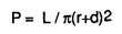
Charts relating soil strength (as measured with a vane shear device) to axle load and ballast thickness are shown in Figure 56 through 58. Figure 56 is based on a single axle, single wheel load. Figure 57 is based on a double wheel, single axle toad, and Figure 58 is based on a tandem wheel configuration typical of 3 axle dump trucks or stinger type log-trucks.

It should be noted that axle and wheel configuration have a tremendous impact on the load bearing capacity of a road. The relationship between axle load and subgrade failure is not linear. Allowing 16,000 kg axle load vehicle to use a road designed for a standard axle load of 8,200 kg, is equivalent to 15 trips with the 8,200 kg axle load vehicle. Premature rut formation and its prevention depends on the selection of the proper axle load and strict enforcement of the selected load standard.

Some typical truck configurations, gross vehicle weights (GVW), and axle or wheel loads are given in Table 24. Vehicles under 3 tonnes GVW have no measurable effect on subgrade stress and deterioration.

Design Example

A road is to be constructed to access a watershed. Because of erosive conditions and traffic volumes, only 5 cm of rutting can be tolerated. Expected traffic volume is high (greater than 1,000 axle loads).

Three vehicle types are using the road:

1. Utility truck - 10 tonnes GVW; 4,500 kg single wheel load (9,000 kg axle load on rear axle, loaded).

2. Dump truck -15 tonnes GVW with two axles; (11 tonnes rear axle load or 5.5 tonnes per dual wheel).

3. Log truck - 36 tonnes GVW with 5 axles, rear tandem axle load equals 15.9 tonnes or 7.95 tonnes per tandem wheel set.

Soil tests: Visually segment the road into logical construction segments based on soil type. Take soil strength measurements with vane shear device. Measurements should be taken during wet soil conditions, its weakest state. Take at least 10 vane shear readings at approximately 10 cm and 40 cm below the surface (in mineral soil). Tabulate readings in descending order from largest to smallest value. Your design shear strength is the 25th percentile shear strength--the value at which 75 percent of the soil strength readings are higher.

Subgrade strength for design purpose is taken as 0.36 kg/cm².

Ballast Depth Calculation: Calculate the soil stress value without fabric for little rutting (less than 5 cm for more than 1,000 axle loads).

q = 2.8 * 0.36 = 1.01 kg/cm²

(Conversion factor: Multiply kg/cm² by 14.22 to get psi. This gives a value of 14.33 psi in this example).

In the case of the utility truck with 4,500 kg (10,000 Ibs) wheel load, enter Figure 56 at 14.33 on the bottom line and read upwards to the 4,500 kg (10,000 Ibs) single wheel load. A reading of 42 cm (16.5 in.) is obtained. Since 7 - 12 cm additional ballast is needed to compensate for intrusion from the soft subgrade, a total of 49 - 54 cm of ballast is required. When fabric is used, a factor of 5.0 (little rutting for high traffic volumes) is applied to determine the ballast depth.

q = (5.0 * 0.36 * 14.22) + 25.6 psi

A reading of 28 cm (11 in.) is obtained from Figure 56 indicating a saving of 21-26 cm of rock when fabric is used.

The same analysis is carried out for the other vehicles. Ballast depth required to support the other vehicles is shown in Table 24.

Table 24. Required depth of ballast for three design vehicles. Road designed to withstand large traffic volumes ( > 1,000 axle loads) with less than 5 cm of rutting.

The dump truck (15 t GVW) represents the most critical load and requires 52 cm of rock over the subgrade to provide an adequate road surface. If fabric were to be used, the utility truck (10 t GVW) would be the critical vehicle. The rock requirement would be reduced by 21 cm to 31 cm. A cost analysis would determine if the cost of fabric is justified.

The above example shows that a simple, 2 axle truck can stress the subgrade more than a 36 tonne log truck. The engineer should consider the possibility and frequency of overloading single-axle, single wheel trucks. Overloading a 4,500 kg (10,000 Ibs) single wheel load truck to 6,750 kg (15,000 lb) increases the the rock requirements from 51 to 62 cm.

Figure 56. Ballast thickness curves for single wheel loads (from Steward, et al., 1977).
Conversion factors: 1 inch = 2.5 cm ; 1 kg/cm² = 14.22 psi.
Multiply (kg / cm²) with 14.22 to get (PSI)

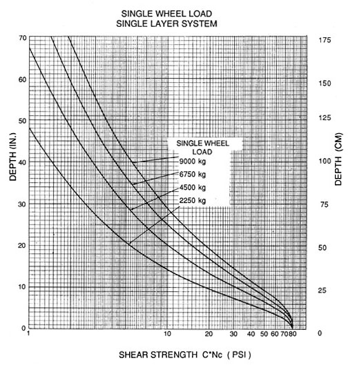
Figure 57. Ballast thickness curves for dual wheel loads (from Steward, et al., 1977).
Conversion factors: 1 inch = 2.5 cm ; 1 kg/cm² = 14.22 psi.
Multiply (kg / cm²) with 14.22 to get (PSI)

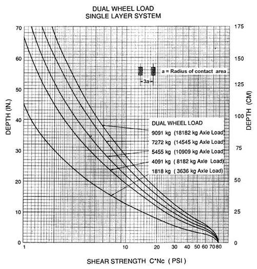
Figure 58. Ballast thickness curves for tandem wheel loads (form Steward et al 1977).
Conversion factors: 1 inch = 2.5 cm; 1 kg/cm² = 14.22 psi.
Multiply (kg / cm²) with 14.22 to get (PSI)

LITERATURE CITED

Armstrong, C. L. 1984. A method of measuring road surface wear. ETIS, Vol. 16, p. 27-32.

Atkins, H. N. 1980. Highway materials, soils, and concretes. Prentice-Hall Co., Reston, VA. 325 p.

Barenberg, E. J., J. Dowland, H. James and J. H. Hales. 1975. Evaluation of Soil Aggregate Systems with Mirafy Fabrics. UIL-ENG-75-2020. University o f Illinois, Urbana - Champaign, Illinois.

Bishop, A. W. 1950. Use of the slip circle inslope stability analysis. Geotechnique 5(1):7-17.

Burroughs, Jr., E. R., G. R. Chalfant and M. A. Townsend. 1976. Slope stability in road construction. U. S. Dept. of Interior, Bureau of Land Management and Montana State University. Portland, Oregon. 102 p.

Burroughs , Jr.,E. R., F. J. Watts and D.F. Haber. 1984. Surfacing to reduce erosion of forest roads built in granitic soils. In: Symposium on effects of forest landslides on erosion and slope stability. May 1984. University of Hawaii, p. 255 - 264.

Cain, C. 1981. Maximum grades for log trucks on forest roads. Eng. Field Notes. Vol. 13, No. 6, 1981. USDA Forest Service, Eng. Techn. Inf. Syst., Washington D.C.

Cain, C. and J. A. Langdon. 1982: A guide for determining road width on curves for single-lane forest roads. Eng. Field Notes. Vol. 14, No. 4-6, 1982. USDA Forest Service, Eng. Techn. Inf. Syst., Washington D.C.

Chen, W. F. and M. W. Giger. 1971. Limit analysis of stability of slopes. J. Soil Mechanics and Foundations Div., Proc. ASCU, Vol. 97, No. Sm1, Proc. Paper 7828, Jan. 1971, pp. 19-26.

Dietz, R., W. Knigge and H. Loeffler, 1984. Walderschliessung. Verlag Paul Parey, Hamburg, Germany, pp. 426.

Kochenderfer, J. N. and J. D. Helvey. 1984. Soil losses from a minimum-standard truck road constructed in the Appalachians. In: Mountain Logging Symposium (ed. P. Peters and J. Luchok) West Virginia University. Morgantown, W. Virginia. p. 215-275.

Kraebel, C. 1936. Erosion control on mountain roads. USDA Circular No. 380, Washington D. C. 44 pp.

Kramer, B. 1982. Vehicle tracking simulation techniques for low speed forest roads in the Pacific Northwest. ASAE No. PNR - 82 - 508. St. Joseph, Michigan.

Kuonen, V. 1983. Wald-und Gueterstrassen Eigenverlag, Pfaffhausen, Switzerland. 743 pp.

Ohmstede, R. 1976. Vertical curves and their influence on the performance of log trucks. Eng. Field Notes. Vol. 8, No. 11, 1976. USDA Forest Service, Eng. Techn. Inf. Syst., Washington D.C.

Pearce, J. K. 1960. Forest Engineering Handbook. Prepared for U. S. Department of the Interior, Bureau of Land Management. 220 pp.

Prellwitz,R. W. 1975. Simplified slope design for low volume roads in mountaineous areas. in: Low volume roads. Proceedings, June 1975. Special Report 160. Transp. Research Board, National Academy of Sciences, Washington, D.C., pp. 65-74.

Reid, L. M. 1981. Sediment production from gravel-surfaced forest roads, Clearwater Basin, Washington. Publ. FRI-UW-8108, Univ. of Washington, Seattle. 247 p.

Reid, L. M. and T. Dunne. 1984. Sediment production from forest road surfaces. Water Resources Research 20:1753-61.

Steward, J. E., R. Williamson, and J. Mohney. 1977. Guidelines for use of fabrics in construction and maintenance of low volume roads. Nat. Tech. Info. Svc. Springfield, VA 22161. 172 pp.

USDA, Forest Service. 1973. Transportation Engineering Handbook, Slope design guide. Handbook No. 7709.11.