ARE COMMODITY PRICES STATIONARY?
The issue of whether agricultural commodity prices are non-stationary is at the crux of the debate regarding responses to cope with price volatility. Although the majority of the empirical evidence favours non-stationarity in prices; - Cuddington, (1992), Cashing, Liang and McDermott, (1999), etc.; others have inferred that prices are stationary: - Powell, 1991, with some having mixed results (Sarris, 1998, 2000). Leon and Soto (1995) found that real commodity prices were non-stationary but once the possibilities of structural breaks were accounted for the series they considered appeared stationary. This result is not unexpected, since the non-stationary behaviour of prices arises as a direct consequence of structural changes and other types of shock which renders commodity markets unstable. This issue is important because it provides an indication of the nature of shocks to commodity prices. Knowledge of whether shocks have a temporary or permanent effect is an essential input in the design of policies to dampen their effects. The available empirical evidence is very difficult to compare and make a clear judgment on, as dates used, the commodity aggregates and the types of commodity prices are all different.
In our analysis, both real and nominal commodity prices were tested for stationarity[22] for each decade. We performed the following widely used unit root tests: the Dickey-Fuller (DF) and augmented Dickey-Fuller (ADF) tests. In addition, a seasonal DF test was carried also out. Each of the tests takes the unit root as the null hypothesis. If the series is correlated at higher order lags, the assumption of white noise disturbances is violated. The ADF test uses a different method to account for higher-order serial correlation in the series. The battery of test used provided mixed results and as a result we did not rely on them to make inference about the stationarity in prices[23]. Rather we computed the modulus of the eigenvalues of the autoregressive characteristic polynomials and examine them to see if they are greater or less than unity.
We computed these roots of up to the 4th order AR characteristic polynomials for all our price series and examined the modulus of the eigenvalues to infer stationarity in our commodity prices. The moduli of all the polynomial roots were found to be close to unity and as a result, we conclude that for all the three decades, prices where non-stationary. The implication of these results is that the effect of shocks to commodity prices persists for some time before they die out. In addition, simple differencing did not render our prices stationary in many cases. We then used several variance stabilizing transformations on a subset of the commodity prices. Among these, the Box-Cox power transformation for values of between (-1, 1) was successful in making these price stationary. Table 2 gives the modulus of the AR characteristic polynomials for selected commodities.
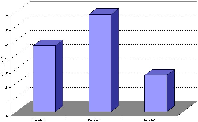
Tests for the degree of persistence of shocks to commodity prices were examined by analyzing the autocorrelation functions of all our commodity prices in both nominal and real terms. Figure 3 shows the extent of the average persistence of shocks across commodities. The figure shows that for the set of commodity prices considered in this study, decade 3 represents the period of relatively rapid adjustments in prices while decade 2 was a period in which it took longer for prices to adjust to their equilibrium levels. This was a period of high levels of protection which in part may explain the persistence of effects of the shocks over a longer time period, which seems to support the position of Deaton and Laroque (1992).
Table App. VII-1: Roots of the Autoregressive (AR) Characteristics Polynomial
|
Commodity |
Real roots |
Modulus |
|
Maize -n |
0.999350 |
0.999400 |
|
Maize -r |
0.915300 |
0.915300 |
|
Palmoil -n |
1.000030 |
1.000000 |
|
Palmoil -r |
0.918450 |
0.918400 |
|
Rapeoil -n |
0.999800 |
0.999800 |
|
Rapeoil -r |
0.908770 |
0.908800 |
|
Rapeseed -r |
1.000090 |
1.000100 |
|
Rapeseed -n |
0.908590 |
0.908600 |
|
Soybean -n |
0.999580 |
0.999600 |
|
Soybean -r |
0.910280 |
0.910300 |
|
Wheat -n |
0.999820 |
0.999800 |
|
Wheat -r |
0.917170 |
0.917200 |
|
Soymeal -n |
0.999000 |
0.999500 |
|
Soymeal -r |
0.910920 |
0.910900 |
|
Rice -n |
0.999660 |
0.999700 |
|
Rice -r |
0.919170 |
0.919200 |
|
Cocoa -n |
0.997090 |
0.997100 |
|
Cocoa -r |
0.914700 |
0.914700 |
|
Coffee -n |
0.992150 |
0.992100 |
|
Coffee-r |
0.924540 |
0.924500 |
|
Sugar -n |
0.998760 |
0.998800 |
|
Sugar -r |
0.928040 |
0.928000 |
|
Cotton -n |
0.997260 |
0.997300 |
|
Cotton -r |
0.924500 |
0.924500 |
|
Jute-n |
0.990340 |
0.990300 |
|
Jute -r |
0.926400 |
0.926400 |
|
Sisal -n |
0.997570 |
0.997600 |
|
Sisal -r |
0.914890 |
0.914900 |
|
Rubber -n |
0.916190 |
0.916200 |
|
Rubber -r |
1.000000 |
1.000000 |
|
Banana -n |
0.973780 |
0.973800 |
|
Banana -r |
0.905970 |
0.906000 |
|
Tea -n |
0.997660 |
0.997700 |
|
Tea -r |
0.901900 |
0.901900 |
Note: The modulus are the absolute eigenvalues regardless of the sign.
The underscore letters n and r refer to nominal and real prices, respectively.
Figure App-VII. 1: Persistence of Shocks across Commodities, by decade

|
[22] Detailed description of
these tests can be found in most standard econometric books. [23] Sarris, 1998, 2000 found the tests inconclusive for cereal prices. |