CHAPTER 4

DRAINAGE DESIGN

4.1 General Considerations

Roads will affect the natural surface and subsurface drainage pattern of a watershed or individual hillslope. Road drainage design has as its basic objective the reduction and/or elimination of energy generated by flowing water. The destructive power of flowing water, as stated in Section 3.2.2, increases exponentially as its velocity increases. Therefore, water must not be allowed to develop sufficient volume or velocity so as to cause excessive wear along ditches, below culverts, or along exposed running surfaces, cuts, or fills.

Provision for adequate drainage is of paramount importance in road design and cannot be overemphasized. The presence of excess water or moisture within the roadway will adversely affect the engineering properties of the materials with which it was constructed. Cut or fill failures, road surface erosion, and weakened subgrades followed by a mass failure are all products of inadequate or poorly designed drainage. As has been stated previously, many drainage problems can be avoided in the location and design of the road: Drainage design is most appropriately included in alignment and gradient planning.

Hillslope geomorphology and hydrologic factors are important considerations in the location, design, and construction of a road. Slope morphology impacts road drainage and ultimately road stability. Important factors are slope shape (uniform, convex, concave), slope gradient, slope length, stream drainage characteristics (e.g., braided, dendritic), depth to bedrock, bedrock characteristics (e.g., fractured, hardness, bedding), and soil texture and permeability. Slope shape (Figure 59) gives an indication of surface and subsurface water concentration or dispersion. Convex slopes (e.g., wide ridges) will tend to disperse water as it moves downhill. Straight slopes concentrate water on the lower slopes and contribute to the buildup of hydrostatic pressure. Concave slopes typically exhibit swales and draws. Water in these areas is concentrated at the lowest point on the slope and therefore represent the least desirable location for a road.

Hydrologic factors to consider in locating roads are number of stream crossings, side slope, and moisture regime. For example, at the lowest point on the slope, only one or two stream crossings may be required. Likewise, side slopes generally are not as steep, thereby reducing the amount of excavation. However, side cast fills and drainage requirements will need careful attention since water collected from upper positions on the slope will concentrate in the lower positions. In general, roads built on the upper one-third of a slope have better soil moisture conditions and, therefore, tend to be more stable than roads built on lower positions on the slope.

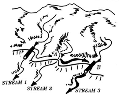
Natural drainage characteristics of a hillslope, as a rule, should not be changed. For example, a drainage network will expand during a storm to include the smallest depression and draw in order to collect and transport runoff. Therefore, a culvert should be placed in each draw so as not to impede the natural disposition of stormflow. Culverts should be placed at grade and in line with the centerline of the channel. Failure to do this often results in excessive erosion of soils above and below the culvert. Also, debris cannot pass freely through the culvert causing plugging and oftentimes complete destruction of the road prism. Headwater streams are of particular concern (point A, Figure 60) since it is common to perceive that measurable flows cannot be generated from the moisture collection area above the crossings. However, little or no drainage on road crossings in these areas is notorious for causing major slide and debris torrents, especially if they are located on convex slope breaks.

Increased risks of road failures are created at points A and B. At point A, water will pond above the road fill or flow downslope through the roadside ditch to point B. Ponding at A may cause weakening and/or erosion of the subgrade . If the culvert on Stream 1 plugs, water and debris will flow to point A and from A to B. Hence, the culvert at B is handling discharge from all three streams. If designed to minimum specifications, it is unlikely that either the ditch or the culvert at B will be able to efficiently discharge flow and debris from all three streams resulting in overflow and possible failure of the road at point B.

Figure 59. Slope shape and its impact on slope hydrology. Slope shape determines whether water is dispersed or concentrated. (US Forest Service, 1979).

A road drainage system must satisfy two main criteria if it is to be effective throughout its design life:

1. It must allow for a minimum of disturbance of the natural drainage pattern.

2. It must drain surface and subsurface water away from the roadway and dissipate it in a way that prevents excessive collection of water in unstable areas and subsequent downstream erosion.

The design of drainage structures is based on the sciences of hydrology and hydraulics-the former deals with the occurrence and form of water in the natural environment (precipitation, streamflow, soil moisture, etc.) while the latter deals with the engineering properties of fluids in motion.

Figure 60. Culvert and road locations have modified drainage patterns of ephemeral streams 2 and 3. Locations A and B become potential failure sites. Stream 3 is forced to accept more water below B due to inadequate drainage at A.

4.2 Estimating runoff

Any drainage installation is sized according to the probability of occurrence of an expected peak discharge during the design life of the installation. This, of course, is related to the intensity and duration of rainfall events occurring not only in the direct vicinity of the structure, but also upstream of the structure. In snow zones, peak discharge may be the result of an intense warming period causing rapid melting of the snowpack.

In addition to considering intensity and duration of a peak rainfall event, the frequency, or how often the design maximum may be expected to occur, is also a consideration and is most often based on the life of the road, traffic, and consequences of failure. Primary highways often incorporate frequency periods of 50 to 100 years, secondary roads 25 years, and low volume forest roads 10 to 25 years.

Of the water that reaches the ground in the form of rain, some will percolate into the soil to be stored until it is taken up by plants or transported through pores as subsurface flow, some will evaporate back into the atmosphere, and the rest will contribute to overland flow or runoff. Streamflow consists of stored soil moisture which is supplied to the stream at a more or less constant rate throughout the year in the form of subsurface or groundwater flow plus water which is contributed to the channel more rapidly as the drainage net expands into ephemeral channels to incorporate excess rainfall during a major storm event. The proportion of rainfall that eventually becomes streamflow is dependent on the following factors:

1. The size of the drainage area. The larger the area, the greater the volume of runoff. An estimate of basin area is needed in order to use runoff formulas and charts.

2. Topography. Runoff volume generally increases with steepness of slope. Average slope, basin elevation, and aspect, although not often called for in most runoff formulas and charts, may provide helpful clues in refining a design.

3. Soil. Runoff varies with soil characteristics, particularly permeability and infiltration capacity. The infiltration rate of a dry soil, by nature of its intrinsic permeability, will steadily decrease with time as it becomes wetted, given a constant rainfall rate. If the rainfall rate is greater than the final infiltration rate of the soil (infiltration capacity), that quantity of water which cannot be absorbed is stored in depressions in the ground or runs off the surface. Any condition which adversely affects the infiltration characteristics of the soil will increase the amount of runoff. Such conditions may include hydrophobicity, compaction, and frozen earth.

A number of different methods are available to predict peak flows. Flood frequency analysis is the most accurate method employed when sufficient hydrologic data is available. For instance, the United States Geological Survey has published empirical equations providing estimates of peak discharges from streams in many parts of the United States based on regional data collected from "gaged" streams. In northwest Oregon, frequency analysis has revealed that discharge for the flow event having a 25-year recurrence interval is Most closely correlated with drainage area and precipitation intensity for the 2-year, 24-hour storm event. This is, by far, the best means of estimating peak flows on an ungaged stream since the recurrence interval associated with any given flow event can be identified and used for evaluating the probability of failure.

The probability of occurrence of peak flows exceeding the design capacity of a proposed stream crossing installation should be determined and used in the design procedure. To incorporate this information into the design, the risk of failure over the design life must be specified. By identifying an acceptable level of risk, the land manager is formally stating the desired level of success (or failure) to be achieved with road drainage structures. Table 25 lists flood recurrence intervals for installations in relation to their design life and probability of failure.

Table 23. Flood recurrence interval (years) in relation to design life and probability of failure.* (Megahan, 1977).

EXAMPLE: If a road culvert is to last 25 years with a 40% chance of failure during the design life, it should be designed for a 49-year peak flow event (i.e., 49-year recurrence interval).

When streamflow records are not available, peak discharge can be estimated by the "rational" method or formula and is recommended for use on channels draining less than 80 hectares (200 acres):

Q = 0.278 C i A

(In English units the formula is expressed as:

Q = C i A

The runoff coefficient, C, expresses the ratio of rate of runoff to rate of rainfall and is shown below in Table 26. The variable tc is the time of concentration of the watershed (hours).

Table 26. Values of relative imperviousness for use in rational formula. (American Iron and Steel Institute, 1971).

Numerous assumptions are necessary for use of the rational formula: (1) the rate of runoff must equal the rate of supply (rainfall excess) if train is greater than or equal to tc; (2) the maximum discharge occurs when the entire area is contributing runoff simultaneously; (3) at equilibrium, the duration of rainfall at intensity I is t = tc; (4) rainfall is uniformly distributed over the basin; (5) recurrence interval of Q is the same as the frequency of occurrence of rainfall intensity I; (6) the runoff coefficient is constant between storms and during a given storm and is determined solely by basin surface conditions. The fact that climate and watershed response are variable and dynamic explain much of the error associated with the use of this method.

Manning's formula is perhaps the most widely used empirical equation for estimating discharge since it relies solely on channel characteristics that are easily measured. Manning's formula is:

Q = n-1 A R2/3 S1/2

(In English units, Manning's equation is:

Q = 1.486 n-1 A R2/3 S1/2

Values for Manning's roughness coefficient are presented in Table 27.

Table 27. Manning's n for natural stream channels (surface width at flood stage less than 30 m) (Highway Task Force, 1971).

Figure 61. Determining high water levels for measurement of stream channel dimensions.

Area and wetted perimeter are determined in the field by observing high water marks on the adjacent stream banks (Figure 61). Look in the stream bed for scour effect and soil discoloration. Scour and soil erosion found outside the stream channel on the floodplains may be caused by the 10-year peak flood. Examining tree trunks and brush in the channel and floodplain may reveal small floatable debris hung up in the vegetation. Log jams are also a good indication of flood marks because their age can be estimated and old, high log jams will show the high watermark on the logs. The difficulty in associating high water marks with flow events of a specified recurrence interval makes values obtained by this method subject to gross inaccuracy. If the 10-year flood can be determined, flow levels for events with a higher recurrence interval can be determined roughly from Table 28.

Table 28. Relationship of peak flow with different return periods. (Nagy, et al, 1980).

A key assumption in the use of Manning's equation is that uniform steady flow exists. It is doubtful that high gradient forested streams ever exhibit this condition. (Campbell, et al., 1982) When sufficient hydrologic data is lacking, however, Manning's equation, together with observations of flow conditions in similar channels having flow and/or precipitation records, provide the best estimate of stream discharge for purposes of designing stream crossings. An example illustrating the use of Manning's equation to calculate peak discharge is as follows:

EXAMPLE: A trapezoidal channel of straight alignment and uniform cross section has a bottom width of 10 meters, side slopes 1:1, channel slope 0.003, and high water depth (25-year event) of 5 meters. The channel has weeds and heavy brush along its banks.

1. The wetted perimeter is equal to 10 + 2(5 / cos 45°) = 24.1 m.

2. The cross sectional area is equal to 1/2 x sum of parallel sides x perpendicular height = 0.5(10 + 20)(5) = 75 m².

3. The hydraulic radius is cross sectional area + wetted perimeter = 75 / 24.1 = 3.1 m.

4. Manning's n from Table 25 is n = 0.06

5. Discharge, Q, from Manning's equation = (0.06)-1 (75)(3.1)2/3 (0.003)1/2 = 146 m3/sec
(Velocity, if needed, can be computed by Q / A = 1.9 m/sec.)

4.3 Channel Crossings

4.3.1 Location of Channel Crossings

Channel crossings require careful design and construction. Functionally, they must (1) allow for passage of the maximum amount of water which can reasonably be expected to occur within the lifetime of the structure and (2) not degrade water quality or endanger the structure itself or any downstream structures. It should be pointed out that most road failures are related to inadequate water passage structures and fill design and placement as well as poor construction practices in such locations.

Accelerated erosion brought about by failure of channel crossing structures can be caused by:

1. Inadequate design to handle peak flow and debris. Water will back up behind structure, saturating the fill and creating added hydrostatic pressure. Water will overflow the structure and the fill may be washed out.

2. Inadequate outlet design. By constricting flow through a small area, water velocity (along with its erosive power) will increase. Outlets need to be properly designed in order to withstand high flow velocities and thus avoid excessive downstream erosion and eventual road failure.

3. Poor location of crossing. Crossings need to be located along relatively stable stretches where stream bottoms and banks exhibit little signs of excessive erosion or deposition. Meandering and/or multiple channels often indicate unstable conditions. If there is no choice but to use a poor location, careful consideration of the type of crossing selected, along with bank and stream bottom stabilization and protection measures, should be given.

There are three generally accepted methods used to cross channels on low volume roads--bridges, fords, and culverts. The selection is based on traffic volume and characteristics, site conditions (hydrologic/hydraulic conditions of channel), and management needs such as occasional closure, continuous use, safety considerations, resource impact (fish, wildlife, sediment). Factors to consider when selecting a crossing type are listed as follows:

1. Bridges: high traffic volume, large and variable water volume, high debris-potential, sensitive channel bottom and banks, significant fish resource, large elevation difference between channel and road grade

2. Culvert: Medium to low water volume, medium to low debris potential, fish resource not significant, elevation difference between channel and road grade less than 10 meters, high traffic volume

3. Ford: low to intermittent water flow, high debris potential, no fish resource, road grade can be brought down to channel bottom, low traffic volume

All three channel crossing types require a careful analysis of both vertical and horizontal alignment. In particular, careful analysis of curve widening requirements is imperative in relation to the specified critical vehicle. Channel crossings are fixed structures where the road way width cannot be temporarily widened. Road width, curvature, approach, and exit tangents govern the vehicle dimensions which can pass the crossing.

Except for bridge locations, roads should climb away from channel crossings in both directions wherever practical so high water will not flow along the road surface. This is particularly true for ford installations.

4.3.2 Fords

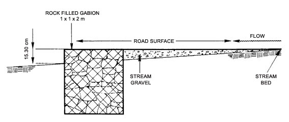
Fords are a convenient way to provide waterway crossing in areas subject to flash floods, seasonal high storm runoff peaks, or frequent heavy passage of debris or avalanches. Debris will simply wash over the road structure. After the incident, some clearing may be necessary to allow for vehicle passage. Figure 62 shows a very simple ford construction where rock-filled gabions are used to provide a road bed through the stream channel.

Figure 62. Ford construction stabilized by gabions placed on the downstream end. (Megahan, 1977).

There are some design considerations which need careful attention:

1. The ford should allow for passage of debris and water without diverting it onto the road surface. The ford results in a stream bed gradient reduction. Therefore, debris has a tendency to be deposited on top of a ford because of reduced flow velocity.

2. Fords should be designed with steep, short banks which help to confine and channel the stream (Figure 63). The steepness and length of the adverse grade out of ford depends on the anticipated debris and water handling capacity required as well as vehicle geometry (See Chapter 3.1.3). Typically, the design vehicle should be able to pass the ford without difficulty. Critical vehicles (vehicles which have to use the road, but only very infrequently) may require a temporary fill to allow passage.

Figure 63. Profile view of stream crossing with a ford. A dip in the adverse grade provides channeling preventing debris accumulation from diverting the stream on to and along the road surface. The profile of the ford along with vehicle dimensions must be considered to insure proper clearance and vehicle passage. (After Kuonen, 1983)

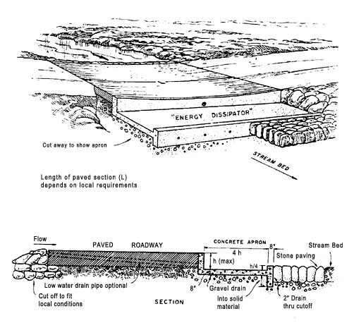
An alternative to the above described ford is a "hardened" fill with culvert (Figure 64). This approach is an attractive alternative for crossing streams which are prone to torrents. The prevailing low flow conditions are handled by a small culvert and the occasional flash flood or debris avalanche will simply wash over the road surface. The fill surface has to be hardened either by concrete or large rock able to withstand the tremendous kinetic energy associated with floods and torrents. Vertical curve design through the stream has to include an adverse grade as discussed for the typical ford.

Figure 64. Hardened fill stream crossings provide an attractive alternative for streams prone to torrents or debris avalanches (Amimoto, 1978).

4.3.3. Culverts

Culverts are by far the most commonly used channel crossing structure used on forest roads. Culvert types normally used, and the conditions under which they are used, areas follows:

Corrugated metal pipe (CMP) ........................................ All conditions except those noted below

CMP with paved invert .................................................. Water carries sediments erosive to metal

CM pipe-arch .............................................................. Low fills; limited head room

Multi-plate .................................................................. Large sizes (greater than 1.8 meters)

Reinforced concrete pipe (RCP) ....................................Corrosive soil or water, as salt water; short haul from plant; unloading and placing equipment available

Reinforced concrete box .............................................. Extra large waterway; migratory fish way

Although more expensive than round culverts, pipe-arch or plate arch types are preferred over ordinary round pipes. Pipe-arch culverts, beers having a more efficient opening per unit area than round pipe for a given discharge, will collect bottom sediments over time when it is installed slightly below the stream grade. They also require lower fills. However, during periods of low flow, water in pipes with this shape may be spread so thin across the bottom that fish passage is impossible. A plate-arch set in concrete footings is the most desirable type from a fish passage standpoint since it has no bottom. The stream can remain virtually untouched if care is exercised during its installation. (Yee and Roelofs, 1980)

Regardless of the type of culvert, they should all conform to proper design standards with regards to alignment with the channel, capacity, debris control, and energy dissipation. They should all perform the following functions:

1. The culvert with its appurtenant entrance and outlet structures should efficiently discharge water, bedload, and floating debris at all stages of flow.

2. It should cause no direct or indirect property damage.

3. It should provide adequate transport of water, debris, and sediment without drastic changes in flow patterns above or below the structure.

4. It should be designed so that future channel, and highway improvements can be made without much difficulty.

5. It should be designed to function properly after fill has settled.

6. It should not cause objectionable stagnant pools in which mosquitoes could breed.

7. It should be designed to accommodate increased runoff occasioned by anticipated land development.

8. It should be economical to build, hydraulically adequate to handle design discharge, structurally durable, and easy to maintain.

9. It should be designed to avoid excessive ponding at the entrance which may cause property damage, accumulation of sediment, culvert clogging, saturation of fills, or detrimental upstream deposits of debris.

10. Entrance structures should be designed to screen out material which will not pass through the culvert, reduce entrance losses to a minimum, make use of velocity of approach insofar as practical, and by use of transitions and increased slopes, as necessary, facilitate channel flow entering the culvert.

11. The outlet design should be effective in re-establishing tolerable non-erosive channel flow within the right-of-way or within a reasonably short distance below the culvert, and should resist undercutting and washout.

12. Energy dissipators should be simple, easy to build, economical and reasonably self-cleaning during periods of low flow.

13. Alignment should be such that water enters and exits the culvert directly. Any abrupt change in direction at either end will retard flow and cause ponding, erosion, or a buildup of debris at the culvert entrance. All of these conditions could lead to failure. (See Figure 65 for suggested culvert-channel alignment configurations and Figure 66 for suggested culvert grades. In practice, culvert grade lines generally coincide with the average streambed above and below the culvert.)

Figure 65. Possible culvert alignments to minimize channel scouring. (USDA, Forest Service, 1971).

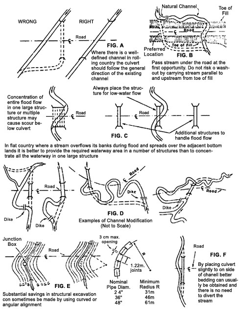
Figure 66. Proper culvert grades. (Highway Task Force, 1971).

If there are existing roads in the watershed, examination of the performance of existing culverts often serves as the best guide to determining the type, size, and accompanying inlet/outlet improvements needed for the proposed stream crossing. For estimating streamflow on many forest watersheds, existing culvert installations may be used as "control sections". Flow can be calculated as the product of water velocity (V) and cross-sectional area (A):

Q = A * V

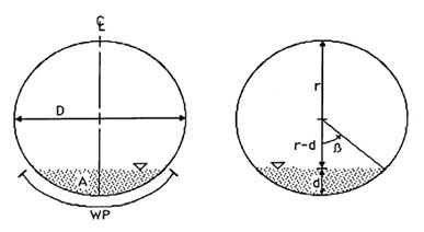
Cross-sectional area of water flowing in a round- culvert is difficult to measure, however a rough estimate can be calculated from the following equation:

Figure 67. Definition sketch of variables used in flow calculations.

Velocity can be calculated using Manning's equation:

V = Q / A = (n-1) (R2/3) (S1/2)

Values for coefficient of roughness (n) for culverts are given in Table 29.

Table 29. Values for coefficient of roughness (n) for culverts. (Highway Task Force,1971).

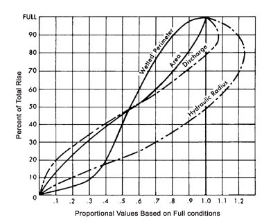
The types of flow conditions found in conventional circular pipes and pipe-arch culverts are illustrated in Figure 68. Under inlet control, the cross-sectional area of the barrel, the inlet configuration or geometry, and the amount of headwater or ponding are of primary importance. Under outlet control, tailwater depth in the outlet channel and slope, roughness, and length of the barrel are also considered. The flow capacity of most culverts installed in forested areas is usually determined by the characteristics of the inlet since nearly any pipe that has a bottom slope of 1.5% or greater will exhibit inlet control. At slopes of 3% or greater, the culvert can become self-cleaning of sediment.

Figure 68. Hydraulics of culverts. (Highway Task Force, 1971).

Once the design peak discharge has been determined by one of the methods discussed above, the size of pipe required to handle the discharge can be determined from available equations, charts, tables, nomographs, etc., such as the ones presented in Figures 70, 71, 72, 73 and 74. Figure 69 provides an example of a work sheet which can be used for diameter and flow capacity calculations. If outlet control is indicated (for example, in a low gradient reach where "backwater effects" may be created at the outlet end), the reader is referred to Handbook of Steel Drainage and Highway Construction Products (1971) or Circular No. 5 published by the U. S. Department of Commerce (1963). Outlet control conditions are shown in Figure 74 for a corrugated metal pipe.

It is important to keep in mind that in addition to discharge from areas upstream of the installation, the culvert must be able to handle accumulated water from roadside ditches recalling that roadside ditches on roads lower on the slope intercept more subsurface water than those on roads higher on the slope. Sudden surges from rapid snowmelt (if applicable) must also be allowed for. Organic debris and bedload sediments can plug a culvert and can greatly reduce culvert efficiency. For these reasons, an "oversized" culvert design may be indicated.

Inlet characteristics can greatly influence flow efficiency through the culvert. The end either (1) projects beyond the fill, (2) is flush with a headwall, or (3) is supplemented with a manufactured mitered steel end section. Inlets with headwalls are generally the most efficient followed by culverts with mitered inlets and finally culverts with projecting entrances. When headwater depths are 1 to 2 times greater than culvert diameter, culverts with headwalls have an increase in flow capacity of approximately 11 and 15%, respectively, over culverts with projecting entrances.

Procedure for Selection of Culvert Size

Note: Culvert design sheets, similar to Figure 69 should be used to record design data.

Step 1: List given data:

a. Design discharge Q, in m3/sec.

b. Approximate length of culvert, in meters.

c. Allowable headwater depth, in meters. Headwater depth is defined as the vertical distance from the culvert invert (flow line) at the entrance to the water surface elevation permissible in the approach channel upstream from the culvert.

d. Type of culvert, including barrel material, barrel cross-sectional shape and entrance type.

e. Slope of culvert. (If grade is given in percent, convert to slope in meters per meter).

f. Allowable outlet velocity (if scour or fish passage is a concern).

g. Convert metric units to english units for use with the nomographs.

Volume flow Q(m3/sec) to Q(cfs) : 1 m3/sec = 35.2 cfs (cubic ft/sec). Multiply Q(m3/sec) by 35.2 to get Q(cfs)

Length, Diameter (meter) : 1 meter = 3.3 ft.; 1 cm = 0.4 inches. Multiply (cm) by 0.4 to get (inches). Multiply (meter) by 3.3 to get (feet)

Step 2: Determine a trial size culvert:

a. Refer to the inlet control nomograph for the culvert type selected.

b. Using an HW/D (Headwater depth/Diameter)) of approximately 1.5 and the scale for the entrance type to be used, find a trial size culvert by following the instructions for use of the nomographs. If a lesser or greater relative headwater depth should be needed, another value of HW/D may be used.

c. If the trial size for the culvert is obviously too large because of limited height of embankment or size availability, try different HW/D values or multiple culverts by dividing the discharge equally for the number of culverts used. Raising the embankment height or using a pipe arch and box culvert which allow for lower fill heights is more efficient hydraulically than using the multiple culvert approach. Given equal end areas, a pipe arch will handle a larger flow than two round culverts. Selection should be based on an economic analysis.

Step 3: Find headwater (HW) depth for the trial size culvert:

a. Determine and record. HW depth by use of the appropriate inlet control nomograph. Tailwater (TW) conditions are to be neglected in this determination. HW in this case is found by simply multiplying HW/D (obtained from the nomograph) by D.

Step 4: Check outlet velocities for size selected:

a. If inlet control governs, outlet velocity can be assumed to equal normal velocity in open-channel flow as computed by Manning's equation for the barrel size, roughness, and slope of culvert selected.

Note: In computing outlet velocities, charts and tables such as those provided by U.S. Army Corp of Engineers, Bureau of Reclamation, and Department of Commerce are helpful (see Literature Cited).

Step 5: Try a culvert of another type or shape and determine size and HW by the above procedure.

Step 6: Record final selection of culvert with size, type, outlet velocity, required HW and economic justification. A good historical record of culvert design, installation, and performance observations can be a valuable tool in planning and designing future installations.

Instructions for Usinq Inlet Control Nomographs

1. To determine headwater (HW):

a. Connect with a straight edge the given culvert diameter or height (D) and the discharge Q, or Q/B for box culverts; mark intersection of straightedge on HW/D scale mark (1).

b. If HW/D scale mark (1) represents entrance type used, read HW/D on scale (1). If some other entrance type is used, extend the point of intersection found in (a) horizontally to scale (2) or (3) and read HW/D.

c. Compute HW by multiplying HW/D by D.

2. To determine culvert size:

a. Given an HW/D value, locate HW/D on scale for appropriate entrance type. If scale (2) or (3) is used, extend HW/D point horizontally to scale (1).

b. Connect point on HW/D scale (1) as found in (a) above to given discharge and read diameter of culvert required.

3. To determine discharge (Q):

a. Given HW and D, locate HW/D on scale for appropriate entrance type. Continue as in 2a.

b. Connect point on HW/D scale (1) as found in (a) above, the size of culvert on the left scale, and read Q or Q/B on the discharge scale.

c. If Q/B is read in (b) multiply by B to find Q.

Good installation practices are essential for proper functioning of culverts, regardless of the material used in the construction of the culvert (Figure 75). Flexible pipe such as aluminum, steel, or polyethylene, requires good side support and compaction, particularly in the larger sizes. It is recommended that the road be constructed to grade or at least a meter above the top of the pipe, the fill left to settle and then excavated to form the required trench.

The foundation dictates if bedding is needed or not. Proper foundation maintains the conduit on a uniform grade. Most times, the culvert can be laid without bedding, however; a few centimeters of bedding helps in installation of the culvert. When bedding is required, the depth should be 8 cm if the foundation material is soil and 30 cm if it is rock.

Backfilling is the most important aspect of culvert installation. Ten percent of the loading is taken by the pipe and 90 percent is taken by the material surrounding the pipe if backfilling is done correctly. Backfill material should consist of earth, sand, gravel, rock or combinations thereof, free of humus, organic matter, vegetative matter, frozen material, clods, sticks and debris and containing no stones greater than 8 cm (3 in) in diameter. It should be placed in layers of no greater than 15 cm (6 in) and compacted up to 95% of Proctor density at or near the optimum moisture content for the material.

Figure 69. Sample work sheet for culvert dimension determination.

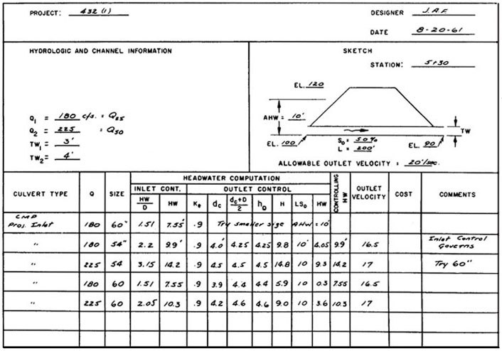
Figure 70. Nomograph for concrete pipes inlet control (U.S. Dept. of Commerce, 1963).

Figure 71. Nomograph for corrugated metal pipe (CMP), inlet control. (U.S. Dept. of Commerce, 1963).

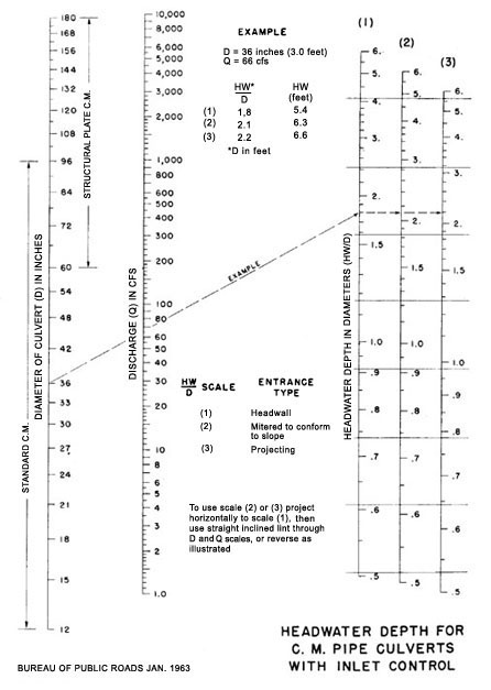
Figure 72. Nomograph for corrugated metal arch pipe (CMP), inlet control. (U.S. Dept. of Commerce, 1963).

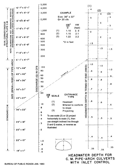
Figure 73. Nomograph for box - culvert, inlet control. (U.S. Dept. of Commerce, 1963).

Figure 74. Nomograph for corrugated metal pipe (CMP), outlet control. (U.S. Dept. of Commerce,1963).

Figure 75. Proper pipe foundation and bedding (1 ft. = 30 cm). (USDA, Forest Service, 1971).

4.3.4 Debris Control Structures

A critical factor in the assessment of channel crossing design and structural capacity is its allowance for handling or passing debris. Past experience has shown that channel crossings have failed not because of inadequate design to handle unanticipated water flows, but because of inadequate allowances for floatable debris which eventually blocked water passage through the culvert. Therefore, each channel crossing has to be analyzed for its debris handing capacity.

When upstream organic debris poses an immediate threat to the integrity of the culvert, several alternatives may be considered.

1. Cleaning the stream of floatable debris is risky and expensive. Since many of the hydraulic characteristics of the channel are influenced by the size and placement of debris, its removal must be carried out only after a trained specialist, preferably a hydrologist, has made a site-specific evaluation of channel stability factors.

2. Various types of mechanical structures (Figures 76, 77 and 78) can be placed above the inlet to catch any debris that may become entrained.

3. A bridge may be substituted in place of a culvert.

Figure 76. Debris control structure--cribbing made of timber.

Figure 77. Debris control structure--trash rack made of steel rail (I-beam) placed over inlet.

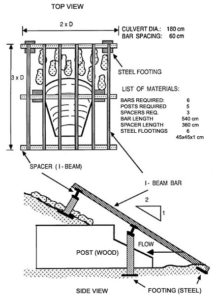
Figure 78. Inlet and outlet protection of culvert with rip-rap. Rocks used should typically weigh 20 kg or more and approximately 50 percent of the rocks should be larger than 0.1 m3 in volume. Rocks can also be replaced with cemented sand layer (1 part cement, 4 parts sand).

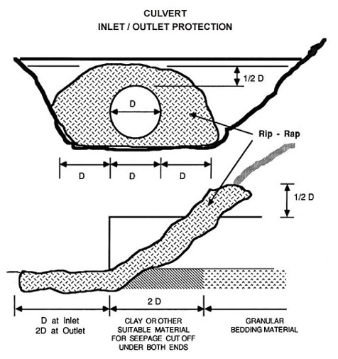
Under high fills, inlets can be provided with upstream protection by rock riprap up to the high water mark (Figure 78). Cambering may also be necessary to ensure the proper grade after fill settlement.

4.3.5. Bridges

Bridges often represent the preferred channel crossing alternative in areas where aquatic resources are extremely sensitive to disturbance. However, poor location of footings, foundations, or abutments can cause channel scour and contribute to debris blockage.

Bridges have been designed using a variety of structural materials for substructure and superstructure. Selection of a bridge type for a specific site should take into consideration the functional requirements of the site, economics of construction at that site, live load requirements, foundation conditions, maintenance evaluations, and expertise of project engineer.

Some arbitrary rules for judging the minimum desirable horizontal and vertical stream clearances in streams not subject to navigation may be established for a specific area based on judgment and experience. In general, vertical clearances should be greater than or equal to 1.5 meters (5 feet) above the 50-year flood level plus 0.02 times the horizontal distance between piers. Horizontal clearance between piers or supports in forested lands or crossings below forested lands should not be less than 85 percent of the anticipated tree height in the forested lands or the lateral width of the 50-year flood. (US Environmental Protection Agency, 1975)

Of course, longer bridge spans will require careful economic evaluations since higher superstructure costs are often involved. Subaqueous foundations are expensive and involve a high degree of skill in the construction of protective cofferdams, seal placement and cofferdam dewatering. In addition to threats to water quality that can occur from a lost cofferdam, time and money losses will be significant. Subaqueous foundations often limit the season of construction relative to water level and relative to fish spawning activity. Thus, construction timing must be rigidly controlled.

It is suggested that the maximum use be made of precast or prefabricated superstructure units since the remoteness of many mountain roads economically precludes bridge construction with unassembled materials that must be transported over great distances. However, the use of such materials may be limited by the capability to transport the units over narrow, high curvature roads to the site, or by the horizontal geometry of the bridge itself.

Another alternative is the use of locally available timber for log stringer bridges. An excellent reference for the design and construction of single lane log bridges is Log Bridge Construction Handbook, by M. M. Nagy, et al., and is published by the Forest Engineering Research Institute of Canada. The reader is referred to this publication for more detailed discussions of these topics.

4.4 Road Surface Drainage

4.4.1 Surface Sloping

Reducing the erosive power of water can achieved by reducing its velocity. If, for practical reasons, water velocity cannot be reduced, surfaces must be hardened or protected as much as possible to minimize erosion from high velocity flows. Road surface drainage attempts to remove the surface water before it accelerates to erosive velocities and/or infiltrates into the road prism destroying soil strength by increasing pore water pressures. This is especially true for unpaved, gravel, or dirt roads.

Water moves across the road surface laterally or longitudinally. Lateral drainage is achieved by crowning or by in- or out- sloping of road surfaces (Figure 79). Longitudinal water movement is intercepted by dips or cross drains. These drainage features become important on steep grades or on unpaved roads where ruts may channel water longitudinally on the road surface.

Figure 79. Road cross section grading patterns used to control surface drainage.

Table 30. Effect of in-sloping on sediment yield of a graveled, heavily used road segment with a 10 % down grade for different cross slopes*

Sloping or crowning significantly reduces sediment delivery from road surfaces. A study by Reid (1981) showed a reduction in sediment delivery by increasing the transverse road surface grade. In this particular case the road surfaces insloped from 5 to 12 percent were compared with conventionally constructed road surfaces at grades of 0 to 2 percent. Sediment yield was reduced by a factor of 3.0 to 4.5 when compared to a conventionally sloped road (Table 30).

Outsloping is achieved by grading the surface at 3 to 5 percent cross slope toward the downhill side of the road. Outsloped roads are simple to build and to maintain. Disadvantages of outsloping include traffic safety concerns and lack of water discharge control. When surfaces become slippery (i.e., snow or ice cover, or when silty or clayey surfaces become wet), vehicles may lose traction and slide toward the downhill edge. Outsloping should only be used under conditions where run-off can be directed onto stable areas. If terrain is less than 20 percent slope and the road gradient is less than 4 percent, outsloping is not an effective way of water removal.

Temporary roads or roads with very light traffic can be outsloped where side slopes do not exceed 40 percent. For safety reasons, when side slopes exceed 40 percent, traffic restrictions should be in force during inclement weather. When outsloping is used for surface drainage, cross drains or dips should be installed on the road surface (Figure 75). Spacing will depend on soil type, road surface and road grade.

Insloping is used where a more reliable drainage system is required such as on permanent roads, roads with high anticipated traffic volumes and/or loads, or in areas with sensitive soils or severe climatic conditions. Insloping is achieved by grading the road surface towards the uphill side of the road at a 3 to 5 percent grade. Water draining from insloped road surfaces is collected and carried along the inside of the road either on the road surface itself or more commonly in a ditch line. The ditch line can be omitted from the road template, thereby reducing the overall road width. This may be desirable in steep terrain in order to reduce excavation (see also Section 3.2). However, this option must be weighed against potential drainage problems along the uphill side of the road. Dips, cross drains, or culverts must be installed and maintained to remove water from the road prism.

Crowned surfaces provide the fastest water removal since the distance water has to travel is cut in half. The crowned surface slopes at 3 to 10 percent from either side of the road centerline. Crowned surfaces and any associated cross drains or dips are difficult to maintain. Water has to be controlled on both sides of the road through a ditch line and stable areas have to be provided for runoff water. Ballast thickness is typically the largest in the center in order to achieve the correct crown shape.

4.4.2 Surface Cross Drains

Cross drains are often needed to intercept the longitudinal, or down-road, flow of water in order to reduce and/or minimize surface erosion. In time, traffic will cause ruts to form, channeling surface water longitudinally down the road. Longitudinal or down-road flow of water becomes increasingly important with:

- increasing grades
- rutting frequency
- road surface protection

Figure 80. Design of outsloped dips for forest roads. A to C, slope about 10 to 15 cm to assure lateral flow; B, no material accumulated at this point - may require surfacing to prevent cutting; D, provide rock rip-rap to prevent erosion; E, berm to confine outflow to 0.5 m wide spillway. (Megahan, 1977).

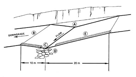
Figure 81. Design of insloped dips for forest roads. A to C, slope about 10 to 15 cm to assure lateral flow; B, no material accumulated at this point - may require surfacing to prevent cutting; D, provide rock rip-rap to prevent erosion; E, berm to prevent overflow; F, culvert to carry water beneath road; G, widen for ditch and pipe inlet (Megahan, 1977).

There are three types of cross drains used for intercepting road surface water: intercept-ing or rolling dips, open top culverts, and cross ditches. Cross drains serve a dual purpose. First they must intercept longitudinal road surface flow, and second they must carry ditch water across the road prism at a frequency interval small enough to prevent concentration of flow. Ditch relief is discussed in more detail in section 4.4.3 and 4.4.4.

Intercepting dips (Figures 80 and 81) when properly constructed, are cheaper to maintain and more permanent than open-top culverts. However, their usefulness is limited to road grades less than 10 percent. At steeper grades, they become difficult to construct and maintain.

Dip locations are determined at the time the grade line is established on the ground or during vertical alignment design. The total length of the two vertical curves comprising the dip should be sufficient to allow the design vehicle to pass safely over them at the design speed. The minimum vertical distance between the crest and sag of the curves should be at least 30 cm (1 ft). It is important that the dip be constructed at a 30 degree or greater angle downgrade and that the dips have an adverse slope on the downroad side. The downroad side of the dip should slope gently downward from the toe of the road cut to the shoulder of the fill. The discharge point of the dip should be armored with rock or equipped with a down-drain to prevent erosion of the fill. Equipment operators performing routine maintenance should be aware of the presence and function of the dips so that they are not inadvertently destroyed.

Open top culverts are most effective on steeper road grades. Open top culverts (Figure 82) can be made of durable treated lumber or poles or they may be prefabricated from corrugated, galvanized steel. The trough should be 7 to 10 cm (3 to 4 in) wide and from 10 to 20 cm (4 to 8 in) deep. The gradient required in order for open top culverts to be self cleaning is 4 percent or greater and, as with dips, they should be angled 30 degrees downslope. In order to maintain their functionality they should be inspected and cleaned on a frequent and regular basis.

Figure 82. Installation of an open-top culvert. Culverts should be slanted at 30 degrees downslope to help prevent plugging. Structure can be made of corrugated steel, lumber or other, similar material. (Darrach, et al., 1982).

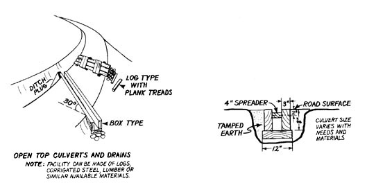
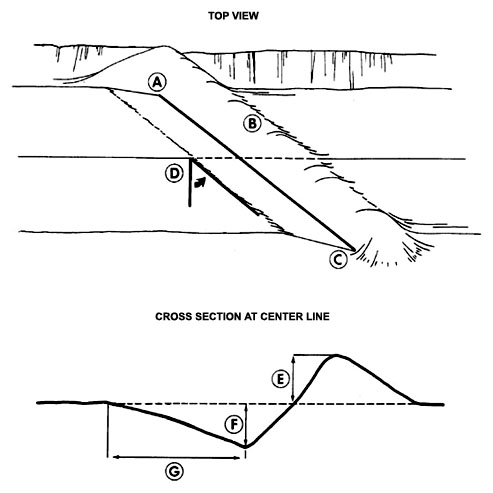
Figure 83. Cross ditch construction for forest roads with limited or no traffic. Specifications are generalized and may be adjusted for gradient and other conditions. A, bank tie-in point cut 15 to 30 cm into roadbed; B, cross drain berm height 30 to 60 cm above road bed; C, drain outlet 20 to 40 cm into road; D, angle drain 30 to 40 degrees downgrade with road centerline; E, height up to 60 cm, F, depth to 45 cm; G, 90 to 120 cm. (Megahan, 1977).

Cross ditches or water bars, are typically used on temporary roads. They are the easiest and most inexpensive method for cross drain installation (Figure 83). However, they impede traffic, wear out quickly, and are difficult to maintain and are, therefore, not recommended except on very low standard roads. In order to be effective, the cross ditch should be excavated into the mineral soil or subgrade and not just into the dirt or surface layer. Water bars should be installed at a 30 degree angle to the centerline of the road, and ditch and berm should be carefully extended to the cut bank in order to avoid ditch water bypass. A berm should be placed in the cut bank ditch to divert water into the cross ditch. Care should be taken that the berm and ditch is not beaten or trampled down by traffic or livestock.

Spacing requirements for surface cross drains depend on road grade, surfacing material, rain intensities, and slope and aspect. Spacing guides for surface cross drains are given in Table 31.

Table 31. Cross drain spacing required to prevent rill or gully erosion deeper than 2.5 cm on unsurfaced logging roads built in the upper topographic position [1] of north-facing slopes [2] having gradient of 80 % [3] (Packer, 1967).

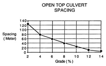
A Japanese open-top culvert spacing guide uses road grade as input (Figure 84) On steep grades, spacing is similar to data given in Table 30. However, on gentler grades (2 - 8%), the Japanese spacing guide provides for considerably wider spacings. This is a good illustration of a case where local conditions take precedent over general guidelines developed for large geographical areas.)

Figure 84. Spacing standard for open-top culverts on forest road surfaces, Japanese Islands. (Minematsu and Minamikata, 1983).

Equal attention must be given to location of cross drains in relation to road and topographic features. Natural features such as slope breaks or ideal discharge locations which disperse water should be identified and incorporated into the drainage plan as needed. Possible locations for cross drains are shown in Figure 85.

Figure 85. Guide for locating cross drains. Several locations require cross drains independent of spacing guides. A and J, divert water from ridge; A, B, and C, cross drain above and below junction; C and D, locate drains below log landing areas; D and H, drains located with regular spacing;. E, drain above incurve to prevent bank cutting and keep road surface water from entering draw; F, ford or culvert in draw; G, drain below inside curve to prevent water from running down road; I, drain below seeps and springs. (Megahan, 1977).

4.4.3 Ditches and Berms

Ditches and berms serve two primary functions on upland roads: (1) they intercept surface run-off before it reaches erodible areas, such as fill slopes, and (2) they carry run-off and sediment to properly designed settling basins during peak flow events (when circumstances warrant the use of settling basins). Ditches and berms are commonly located at the top of cut and fill slopes and adjacent to the roadway, although midslope berms may be useful in controlling sediment on cut and fill slopes before erosion control cover has been established.

The required depth and cross sectional area of a roadside ditch is determined by the slope of the ditch, area to be drained, estimated intensity and volume of run-off, and the amount of sediment that can be expected to be deposited in the ditch during periods of low flow. Triangular or trapezoidal-shaped ditches may be utilized, whichever is appropriate. The ditch cross section is designed so that it will produce the desired water velocity for a given discharge. Minimum full capacity flow velocities should be 0.76 to 0.91 meters/second (2.5 to 3 feet/second) to permit sediment transport. It is best to remember that, in shaping a ditch, given equal grade and capacity, a wide, shallow cross section will generate lower water velocities with correspondingly lower erosion potential than will a narrow, deep cross section. Maximum permissible velocities for unlined ditches of a given soil type are listed in Table 32.

Table 32. Maximum permissible velocities in erodible channels, based on uniform flow in straight, continuously wet, aged channels. For sinuous channels, multiply allowable velocity by 0.95 for slightly sinuous, 0.9 for moderately sinuous, and 0.8 for highly sinuous channels. (U. S. Environmental Protection Agency, 1975).

Table 33. Manning's n for open ditches

Figure 86. Ditch interception near stream to divert ditch water onto stable areas instead of into the stream. (U. S. Environmental Protection Agency,1975).

The procedure for calculating flow rates is the same as that discussed in Section 4.2. The corresponding roughness factors (Manning's n) for open channels are given in Table 33. Ditches in highly erodible soils may require riprap, rock rubble lining, jute matting, or grass seeding. Riprap or rubble-lined ditches will tend to retard flow enough to allow water movement while retaining the sediment load at low flow periods. Lining ditches can reduce erosion by as much as 50 percent and may provide economical benefits by reducing the required number of lateral cross drains when materials can be obtained at low cost.

Ditch water should not be allowed to concentrate, nor should it be allowed to discharge directly into live streams. A cross drain such as a culvert should carry the ditch water across and onto a protected surface (Figure 81). Spacing of ditch relief culverts is discussed in Section 4.4.4 and 4.5.

The ditch grade will normally follow the roadway grade. However, the minimum grade for an unpaved ditch should be 1 percent. Runoff intensity or discharge values needed to calculate ditch size can be determined by calculations described below for culvert design. However, allowances should be made for sedimentation, plus at least 0.3 m between the bottom of the roadway subgrade and the full flow water surface. The suggested minimum size of roadside ditches is shown in Figure 87.

Figure 87. Minimum ditch dimensions.

Velocity of the ditch water is a function of cross section, roughness and grade. For a typical triangular cross section the velocity can be calculated from Manning's equation:

V = n-1 * R2/3 * S1/2

where V equals velocity in meters/second and the other values are as defined in Chapter 4.2. For a triangular channel with sideslopes of 1:1 and 2:1, flowing 0.3 meters deep, the hydraulic radius, R, equals 0.12 m. Table 34 lists ditch velocities as a function of roughness coefficients and grade, and Figure 88 provides a nomograph for the solution of Manning's equation.

In most cases ditch lines should be protected to withstand the erosion. For channels with grades steeper that 10 percent, a combination of cross section widening, surface protection and increased surface roughness may be required.

Table 34. Ditch velocities for various n and grades. Triangular ditch with side slope ratio of 1:1 and 2:1, flowing 0.30 meters deep; hydraulic radius R = 0.12.

Figure 88. Nomograph for solution of Mannin's equation (U.S. Dept. of Commerce, 1965).

EXAMPLE:

Determine whether the water velocity for a road ditch will be below critical levels for erosion. If velocities are too high, make and evaluate changes (see also U.S. Forest Service, 1980). Ditch dimension is a symmetrical, triangular channel, 0.39 m deep with 2.5:1 slopes with sandy banks (SW) and a slope of 0.003 m/m.

Solution:

1. The hydraulic radius, R, is equal to area divided by wetted perimeter.

R = 0.38 m² / 2.1 m = 0.18 m

Converting to english units, divide meters by 0.3 m/ft.

R = 0.60 ft

2. Obtain roughness coefficient from Table 32 (n = 0.020).

3. Obtain maximum allowable velocity 0.46 to 0.76 m/sec (Table 31). Convert to english units by dividing by 0.3 m/ft.

Vmax = 1.5 to 2.5 ft/sec

4. From Figure 88, find the velocity for the specified ditch (2.9 ft/sec). Convert to metric by multiplying by 0.3 m/ft.

Vditch = 0.87 m/sec

5. Compare the calculated ditch velocity with the maximum recommended velocity for sandy channels:

The ditch has too great a velocity given the conditions stated above. Therefore, measures must be taken that will reduce the water velocity. Water velocity in ditches can be reduced by protecting the channel with vegetation, rock, or by changing the channel shape. (With vegetative protection, the friction factor (n) becomes 0.030 - 0.050 and the maximum recommended velocity becomes 0.9 - 1.2 m/sec.)

6. Obtain velocity for specified ditch with vegetative protection by referring to Figure 88 (1.9 feet per second).

7. Compare the calculated ditch velocity with the maximum recommended velocity for vegetation protected channels (average turf) with easily eroded soils:

8. If the specified ditch has a lower velocity than the recommended maximum velocities, it should be stable as long as the vegetation remains intact.

Berms can be constructed of native material containing sufficient fines to make the berm impervious and to allow it to be shaped and compacted to about 90 percent maximum density. Berm dimensions are illustrated in Figure 89.

Figure 89. Minimum berm dimensions.

4.4.4 Ditch Relief Culverts

Water collected in the cutslope ditch line has to be drained across the road prism for discharge at regular intervals. Cross drains should be installed at a frequency that does not allow the ditch flow to approach maximum design water velocities. Intercepting dips or open top culverts (Chapter 4.4.2) perform adequately up to a certain point. However, these techniques are not adequate or appropriate when the following conditions are present either in combination or alone:

- high traffic volumes or loads and characteristic rutting.
- steep side slopes.
- large volumes of ditch water from rainfall,snowfall, springs, or seepage.

Ditch relief culverts do not impact or impede traffic as dips and open-top culverts do. Intercepting dips may become a safety hazard on steep slopes as well as being difficult to construct. It is also undesirable to have large amounts of water running across the road surface because of sediment generation and seepage into the subgrade.

The frequency, location and installation method of ditch relief culverts is much more important than determining their capacity or size. Ditch relief culverts should be designed so that the half-full velocities are 0.7 to 1.0 m/sec in order to transport sediment through the culvert and should be at least 45 cm (18 inches) in diameter depending on debris problems. Larger culverts are more easily cleaned out than narrow ones. Every subsequent relief culvert should be one size larger than the one immediately upstream from it. This way, an added safety factor is built in should one culvert become blocked.

As with dips, open top culverts, and water bars, ditch relief and lateral drain culverts should cross the roadway at an angle greater than or equal to 30° downgrade. This helps insure that water is diverted from the roadside ditch and that sediment will not accumulate at the inlet. Accelerated ditch erosion may (1) erode the road prism making it unstable and unusable, and (2) cause culverts to plug or fail, thereby degrading water quality.

Selection of proper location is as important as spacing. Spacing recommendations should be used as a guide in determining the frequency of cross drain spacing. Final location is dictated by topographic and hydrologic considerations. Considerations discussed for for cross drain locations are also valid for culverts (see Figure 85). Considerations given for stream culvert installation, inlet and outlet protection, should also be used for ditch relief culverts.

Culvert outlets with no outlet protection are very often the cause of later road failures. Normally, culvert outlets should extend approximately 30 - 50 cm beyond the toe of the fill. Minimal protection is required below the outlet for shallow fills. However, on larger fill slopes where the outlet may be a considerable distance above the toe of the fill, a downspout anchored to the fill slope should be used (Figure 90). Culvert outlets should be placed such that at least 50 meters is maintained between it and any live stream. If this is not possible, the rock lining of the outlet should be extended to 6 meters to increase its sediment trapping capacity (Figure 91). Coarse slash should be placed near the outlet to act as a sediment barrier.

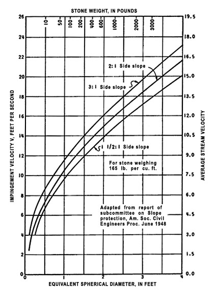
Where fills consist entirely of heavy rock fragments, it is safe to allow culverts to discharge on to the slop. The size and weight of fragments must be sufficient to withstand the expected velocity of the design discharge. Rock aprons (Figure 92) are the least costly and easiest to install. A guide for selecting rock for use as riprap is illustrated in Figure 93.

Figure 90. Ditch relief culvert installation showing the use of headwall, downspout and a splash barrier/energy dissipator at the outlet. Minimum culvert grade is 3 to 5 percent. Exit velocities should be checked. (U. S. Environmental Protection Agency, 1975).

Figure 91. Ditch relief culvert in close proximity to live stream showing rock dike to diffuse ditch water and sediment before it reaches the stream. (U. S. Environmental Protection Agency, 1975).

Figure 92. Energy dissipators. (Darrach, et al., 1981).

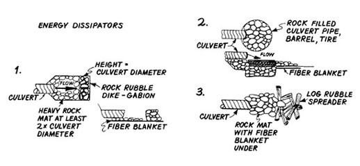
Figure 93. Size of stone that will resist displacement by water for various velocities and ditch side slopes. 1 ft.= 30 cm (U.S. Dept. of Commerce, 1965).

The determination of culvert spacing for lateral drainage across the roadway is based on soil type, road grade, and rainfall characteristics. These variables have been incorporated into a maximum spacing guide for lateral drainage culverts developed by the Forest Soils Committee of the Douglas-fir Region in 1957. The spacing estimates are designed for sections of road 20 feet wide and include average cut bank and ditch one foot deep. Table 2 (Chapter 1.4.1) groups soils by standard soil textural classes into ten erosion classes having erodibility indices from 10 to 100, respectively. (Class I contains the most erodible soils and Class X the least erodible soils.) In order to arrive at an erosion class for a particular soil mixture, multiply the estimated content of the various components by their respective erosion index and add the results.

Example:

The spacing of lateral-drainage culverts can then be obtained from Table 34. The summary equation used to calculate values in Table 34, expressed in metric units, is:

Y = (1,376 e0.0156X )(G R)-1

Values in Table 34 are based on rainfall intensities of 2.5 to 5 cm per hour (1 to 2 in/hr) falling in a fifteen minute period with an expected recurrence interval of 25 years. For areas having greater rainfall intensities for the 25 year storm, divide the values in the table by the following factors:

Roads having grades less than 2 percent have a need for water removal to prevent water from soaking the subgrade or from overrunning the road surface. Thus, spacing for roads with 0.5 percent grades is closer than for roads with 2 percent grades. Usually, local experience will determine the spacing needed for road grades at these levels.

Table 35. Guide for maximum spacing (in feet) of lateral drainage culverts by soil erosion classes and road grade (2% to 18%). (Forest Soils Comm., Douglas Fir Reg., PNW, 1957).

4.5. Subsurface drainage

When groundwater cannot be effectively removed or intercepted by surface drainage, subsurface drainage techniques are required. As discussed in previous sections of this workbook, if water is not removed from subgrade or pavement structures it may create instability, reduce load bearing capacity, increase the danger of frost action and create a safety hazard by freezing of the traveled surface.

Field investigations carried out during the route reconnaissance and design stages may not always reveal subdrainage problems. These less obvious problems can be effectively dealt with during construction. Field investigations should be carried out during the wet season and may include soil and/or geologic studies, borings or trenches to locate groundwater, inspections of natural and cut slopes in the local area, and measurement of discharge when possible. Sites with potential slope stability problems should be more thoroughly evaluated. When groundwater tables approach the ground surface, such as in low, swampy areas, the gradeline should be placed high enough to keep water from being drawn up into the fill by capillary action. Whenever possible, well graded granular materials, such as coarse sand, should be used for fill construction. For a detailed discussion of grading requirements for filter materials the reader is referred to the Earth Manual published by the U.S. Department of the Interior (1974).

Three types of subdrainage systems are commonly used:

(1) Pipe underdrains. This system consists of perforated pipe placed at the bottom of a narrow trench and backfilled with a filter material such as coarse sand. It is generally used along the toes of cut or fill slopes. The trench should be below the groundwater surface and dug into a lower, more inpervious soil layer to intercept groundwater. The drains may be made of metal, concrete, clay, asbestos-cement, or bituminous fiber and should be 15 centimeters (6 inches) in diameter or larger.

(2) Drilled drains. This system consists of perforated metal pipes placed in holes drilled into cut or fill slopes after construction.

(3) French drains. This system consists of trenches backfilled with porous material, such as very coarse sand or gravel. This type of drain is apt to become clogged with fines and is not recommended.

A major difficulty in selecting a drainage system is the lack of adequate performance data for various drainage methods. A good knowledge of seasonal groundwater fluctuations, variation in lateral and vertical permeability, and the ratio of vertical to lateral permeability are critical. Long term monitoring of drainage performance is important in determining appropriate prescriptions for future installations. For example, perforated drains are commonly prescribed but often will not function properly as a result of clogging of pores with fines or from geochemical reactions leading to the formation of precipitates. Several methods may be used to prevent plugging depending on soil characteristics and material availability. The first is to enclose the perforated pipe with geotextile fabric. Second, surround the pipe with an open graded aggregate material, which in turn is surrounded by a fabric. The use of fabric eliminates the need for an inverted filter consisting of various sized gravel and sand layers. Third, if fabric is not available, surround the pipe with a graded aggregate filter. Although the cost of installing such a drainage system is high, it may effectively reduce final road costs by decreasing the depth of base rock needed, thereby reducing subgrade widths and associated costs for clearing, excavating, and maintenance.

LITERATURE CITED

Amimoto, P. Y. 1978. Erosion and sediment control handbook. California Division of Mines and Geology, Department of Conservation. 197 p.

Beschta, R. L. 1981. Streamflow estimates in culverts. Oregon State University, Forest Researph Laboratory, Res. Note. 67. 4 p.

Darrach, A. G., W. J. Sauerwein, and C. E. Halley. 1981. Building water pollution control into small private forest and ranchland roads. U. S. Department of Agriculture, Forest Service and Soil Conservation Service.

Forest Soils Committee of the Douglas Fir Region. 1957. An introduction to the forest soils of the Douglasfir Region of the Pacific Northwest. University of Washington.

Highway Task Force. 1971. Handbook of steel drainage and highway construction products (2nd Ed). American Iron and Steel Institute, 150 E 2nd Street; New York. 368 p.

Megahan, W.F. 1977. Reducing erosional impacts of roads. In: Guidelines for Watershed Management. Food and Agriculture Organization, United Nations, Rome. p 237-261.

Minematsu, H. and Y. Minamikata, 1983. Optimum spacing for open - top culverts on forest roads. University of Agriculture and Technique, Tokyo. Jour. of J.F.S. 65(12):465-470.

Packer, P. 1967. Criteria for designing and locating logging roads to control sediments. Vol.1, No. 13.

Pearce, J. K. 1960. Forest engineering handbook. U. S. Department of Interior, Bureau of Land Management. 220 p.

Reid, L.M. 1981. Sediment production from gravel-surfaced forest roads, Clearwater basin, Washington. Publ. FRI-UW--8108, Univ. of Washington, Seattle. 247 p.

Searcy, J. K. 1967. Use of riprap for bank protection. Federal Highway Administration, Washington D. C. 43 p.

USDA, Forest Service. 1971. Transportation engineering handbook. Handbook No. 7709.11.

________________. 1979. Technical guide, erosion prevention and control on timber sales areas. Intermountain Region.

Yee, C. S. and T. D. Roelofs. 1980. Planning forest roads to protect salmonid habitat. U. S. Department of Agriculture, Forest Service. General Technical Report PNW-109. 26 p.

U.S. Dept. of Commerce, Bureau of Public Roads. 1963. Hydraulic Charts for the Selection of Highway Culverts, Hydraulic Engineering Circular No. 5.

U.S. Dept. of the Interior, Bureau of Reclamation. 1974. Earth Manual, a water resources technical publication. Second edition. Government Printing Office, Washington D.C.