1. Introduction
This annex presents information about the variables used in framing the poverty weighted congruence analysis, sources of data, basic assumptions in framing the poverty indicator, and presents the effects on primary variables of alternative assumptions about values for critical variables. It is divided into four parts: estimating relative values of production, estimating incomes in 1995 and 2010, constructing the poverty indicators, and discussion of results from sensitivity analysis.
2. Estimating relative values of production
FAO quantity and price data were used to estimate the relative values of production for each commodity by country for 1992-94 and 2010. Only those 27 commodities of direct interest to the CGIAR were included in the analysis. For the most part quantity data on the 27 were taken directly from FAO estimates. In some cases, judgments were required as relevant statistics were not available for 2010:
- CGIAR commodities include five pulses (beans, chickpea, cowpea, lentils, pigeonpea). Data on each were available for 1992-94 (1993*) but only projections for the entire set were available for 2010. TAC assumed that the proportions of each in 2010 were like those in 1993*.- As with pulses, sweet potato and yam are shown separately in 1993* but combined for 2010. Again, TAC assumed that the proportions of each in 2010 were like those in 1993*.
- Oil crops were treated as an aggregate and 2010 projections expressed in oil equivalents. Approximate country projections for groundnut, soybean and coconut were derived from production ratios and growth rates.
- As reported 1, the data on fisheries are in terms of utilization and combine products of direct interest to the CGIAR with others that pertain to capital intensive, commercial fishing. TAC made the assumption that 50% of marine catches are generated by commercial enterprises to estimate the production of particular value to the CGIAR. This value is based on informed judgement received from ICLARM and others. TAC assumed that, for the products of direct interest to the CGIAR, utilization and production are equal. Finally, except for China and high income East Asian countries, data on fisheries for 2010 are reported by region only. TAC assumed that regional data adequately represented the sector. In estimating the values, the steps followed tend to overestimate the quantities produced.
1 L. Westlund, 1995. Apparent historical consumption and future demand for fish and fishery products - Exploratory calculations. Paper presented at the International Conference on Sustainable Contribution of Fisheries to Food Security. Kyoto, Japan, 4-9 December 1995. KC/FI/95/TECH/8.
While price data were available for 1993*, estimates for 2010 were available for only a few of the 27 commodities with which the CGIAR deals directly. FAO estimates for relative prices were available for 1989-91 for all but fisheries and forestry. (Prasada Rao, unpublished data, FAO Statistics Division). Unlike any other data set available, these estimates had the great advantage of being based on a consistent format across countries. TAC assumed that relative prices for the crop and livestock commodities would be the same in 2010 as in 1989-91. As no evidently better estimates of international prices were available, TAC also applied the same prices to the 1992-94 quantities to estimate 1993* values of production. Separate estimates, based on current prices were applied to fish and forest products.
Estimating Incomes in 1995 and 2010
The national incomes used in calculating the poverty indicator have all been adjusted for differences in purchasing power parity (PPP). The World Bank Atlas 1996 has estimates of PPP income for 89 countries. UNDP has estimates of PPP income for 1992-94 (based on World Bank data) for virtually all of the remaining countries with significant Agricultural production. As the UNDP estimates are in terms of 1991 PPP income while those of the World Bank are in terms of 1995 PPP income, World Bank estimates of income growth rates from 1985-1994 were used to bring the UNDP estimates to 1995.
Like the estimated value of production, TAC's poverty indicator is based on a projection to 2010. To estimate incomes and poverty levels in 2010, TAC needed income growth rates for each of the countries included in the analysis. After discussion, it was decided to project the PPP incomes of the recent past to 2010. The growth rates used for the income projection stem from the FAO World Agriculture 2010 study. In order to assess the sensitivity of the resulting poverty indicators to the growth rates assumed, TAC compared this model with one in which PPP incomes were assumed to grow 25% less rapidly than estimated by FAO.
Constructing the Poverty Indicators
The poverty indicator is the weight used in modifying the estimated 2010 value of production of each commodity in the analysis. The higher the value of the poverty indicator for a particular country, the more that country's product will count in the total value of product. The consequence is that the products of poorer countries have a larger influence on the relative value of a commodity with the poverty indicator than if it were not applied.
At the end of Chapter 3.8, TAC lists the characteristics desired for its poverty indicator. Its role is to systematically give more weight to the commodities produced in the poorest developing countries. TAC consulted with Martin Ravallion of the World Bank in its development and Ravallion provided materials on which the following descriptive note is based.
|
Box 1: A Measure of Poverty (Based on material from Martin Ravallion, World Bank) In reviewing and rebalancing CGIAR priorities, TAC must ensure that poverty plays a central role. The instrument for incorporating poverty must be consistent with the concerns and pronouncements of the Group, with the level at which TAC sets priorities, with priority setting at the centre and programme level, and with good practice. The key principles are that: 1. the measure for any country should reflect both the average income in the country (negatively) and the degree of inequality (positively); 2. the weight attached to the gains in any one country should be higher the lower the value of the measure for that country; 3. beyond some point the weight should fall to zero; 4. the rate at which the weight increases as the measure of poverty declines and the value of the point beyond which the weight is zero are both matters of judgement, for which it should be easy to assess the extent to which alternative judgements influence the results. To satisfy these principles, the following elements were incorporated: 1. A welfare indicator resting on the distribution-corrected mean income at purchasing power parity. This indicator is given by w = (1-G)y, where G is the Gini index of income or expenditure inequality and y is mean income at purchasing power parity. 2. The poverty indicator has value zero whenever the value of y exceeds some critical value z, for which alternative values are assessed. 3. Whenever w is at or below z, the poverty indicator is given by (1-w/z) raised to the power alpha, where alpha is set at a value of one or higher, and for which alternative values are chosen. |
The indicator has three major parameters. The function of the exponent is to give added weight to the depth of poverty. Increasing the value of the exponent, other things equal, leads to a higher value for the indicator, and, the lower the PPP income, the sharper the increase. Given the discussion in Chapter 3.8, the exponent was set at 2 in the Base Model and raised to 3 for sensitivity analysis.
The function of the Gini Coefficient, 'G', is to adjust for differences among countries in the distribution of income. The Coefficient itself takes on values from zero (indicating that income is equally distributed across the entire population) to one (indicating that all income is in the hands of a single individual). Among the countries included in TAC's analysis, the range is from a low of 0.28 for Bangladesh to 0.60 for Brazil. For a given PPP income, a given value for 'z', and a given value for the exponent, a larger Gini Coefficient leads to a larger poverty indicator. For sensitivity analysis the value of G was divided by 2, reducing the value of the poverty indicator, with stronger effects on higher-income countries than on poorer countries.
The third parameter, 'z', gives the level of PPP income at which the value of the poverty indicator falls to zero when, effectively, the country no longer figures in setting priorities (except as a potential alternative source of supply). The lower the value of 'z' the more countries not figuring in setting priorities and the more impact that the poorest countries have on priorities. The World Bank defines middle income countries as those with an average PPP income above US$ 6000. For the Base Model TAC chose a 'z' of US$ 9000 PPP income and US$ 6000 PPP for sensitivity analysis.
For 'z' at US$ 9000 the following countries are excluded from the analysis and hence do not directly influence CGIAR priorities: (in Asia) Brunei, Malaysia, North Korea, Singapore, South Korea, Taiwan, and Thailand; (in LAC) Argentina, Barbados, Chile, Colombia, Mexico, Panama, Puerto Rico, Trinidad and Tobago, and Venezuela; (in WANA) Bahrain, Cyprus, Kuwait, Oman, Qatar, Saudi Arabia, and United Arab Emirates.
At US$ 6000 the following additional countries are excluded from the analysis: (in SS Africa) Botswana, and Mauritius; (in Asia) China, Indonesia, Papua New Guinea, and Sri Lanka; (in LAC) Belize, Brazil, and Costa Rica; (in WANA) Algeria, Iran, Lebanon, Tunisia, and Turkey.
Note that this approach differs from that taken in the 1996 draft P & S where PPP adjusted for 'G' was the measure compared against 'z'. The present approach gives more emphasis to poor countries. A final point here is that, while countries not included in the analysis do not figure directly in setting CGIAR priorities, they nonetheless will serve as alternative sources of supply, hence will figure in resource allocations, and will have access to all CGIAR products.
The Quantitative Model to Estimate Commodity Priorities
The 2010 values of forecasted production, i.e. the country production volume in tons and the commodity prices in international dollars listed in Table 5, are multiplied by the country poverty indicators described in the section above. As a consequence, the estimated 2010 value of production is weighted by poverty, i.e. the greater the poverty, the higher the weight and the larger the weighted value.
Each commodity produced within a country has the weight associated with that country. Summing across countries for a commodity combines all of the poverty weighted values in a single, global value. Relative to one and other, commodities produced mostly in poor countries tend to gain versus commodities produced mostly in better off countries. For example, in 2010 wheat has 3.5 times the unweighted value of cassava (column 2 in Table 2), while the proportion falls to 2.1 times for the poverty weighted values (column 3 in Table 2). This is a 43% increase in the weighted value of cassava as compared to wheat, manifesting the impact of the poverty indicator.
Finally, changes in the values of the parameters of the poverty indicator change the relative weighted values associated with commodities, sectors, and, especially, regions.
Results from Sensitivity Analysis
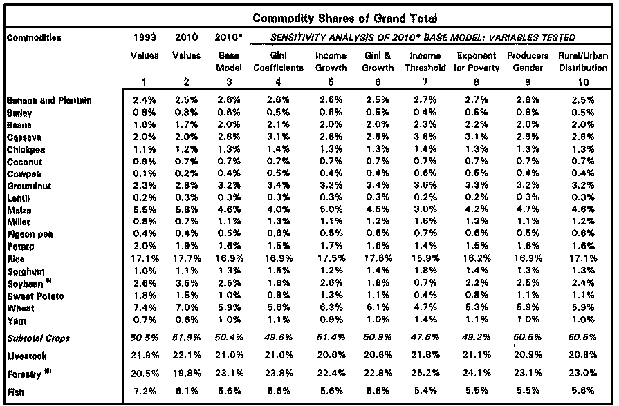
In order to assess the importance of the assumptions made about the key parameters, sensitivity analysis was undertaken. The measure used was the poverty-weighted estimated 2010 value of the commodities with which the CGIAR deals with the exception of forest and fishery products for reasons explained in Chapter 6. The data in the following tables are in terms of percentages, the portion of poverty weighted value associated with that commodity, or sector, or region. By varying the values of the parameters the effect on the proportion can be seen immediately.
In addition to the parameters directly associated with the poverty indicator, sensitivity analysis was also applied to the weights given to female and male producers and to those given to rural and urban residents. In each case the Base Model treats females and males equally and it treats rural and urban dwellers equally. Sensitivity analysis aimed at seeing the effects of giving 25% more weight to females (Column 9) and 25% more weight to rural dwellers (Column 10).
First, note the importance of the poverty indicator itself. This is apparent in Table 3 by comparing Column 2, where unweighted values for estimated 2010 production are the basis for the percentages, with Column 3, where the poverty indicator has had its influence. Note in particular the sharp increase in the portion for Sub Saharan Africa (SSA), up about 50%, and the sharp decrease for Latin America, down about one third.
For commodities, shown in Table 2, the results are not so dramatic. This is because most of the CGIAR commodities are produced in many countries so that gains through the inclusion of the poverty indicator in some countries are offset by loses in others. Even so, there are gains of over 20 percent for cassava, millet, and pulses and, necessarily, losses for several crops, none of them large. Nor are the consequences large in Table 1, where sectors are displayed. Indeed, in Table 1, only the changes in 'z' have consequential implications for the percentages among the sectors.
Decreasing the Gini Coefficient, seen in Column 5 of Table 2, has little influence on commodities but, again has a strong positive influence on SSA and a notably negative influence on LA as seen in Column 5 of Table 3.
Reducing the rate of income growth, seen in Column 6, brings increases to the three major cereals, probably because of the consequent increase of the weight given to production in China, with offsetting losses in such commodities as cassava and pulses. As would be expected, proportions to SSA decline a bit while that for Asia increases. Again, though, the movement is not large in absolute terms, and on the order of 10% in the case of SSA.
Changing the value of 'z', the threshold beyond which the products of a country no longer count directly in priority setting, has a modest effect on crops in Table 1, Column 8, strong negative effects on wheat and maize and strong positive effects on sorghum, millets, pulses, and cassava. Much of this can be attributed to the departure of China from the list, where virtually no cassava, but much maize and wheat, are produced. Regionally SSA gains and all other regions lose, LA notably, as Brazil drops out.
Increasing the exponent, thereby increasing the weight given to the commodities of the poorest countries, has little influence on sectors; it lowers the share of maize, rice, and wheat while increasing that of cassava and pulses. Moreover, it leads to an increase in the share of SSA while decreasing the share of all other regions.
In general, and as would be expected given the structure of the poverty indicator and its influence on the weighted value of production, changes in parameter values that favor the poor push up the shares of the commodities of most relative importance in SSA and, as a result, regional shares move towards SSA. The variable to which the analysis is most sensitive is that related to threshold income, 'z'. Not only does lowering the threshold move some large producers off the list, it reduces the importance of countries at the top of the remaining list, with obvious positive consequences for the poorest countries and their commodities.
Turning now to the two remaining dimensions of sensitivity analysis, increasing the weight given to female producers and to rural populations, the results of sensitivity analysis are in comparing the Base Model of Column 3 with Columns 9 and 10. Looking first at the result of increasing the weight for women, there is little difference for sectors, a modest increase for SSA and, surprisingly, a larger increase for Latin America. As for sectors, the differences from the Base Model are small except for livestock, where the share increases.
Where more weight is given to rural than to urban populations, the livestock sector gains a bit with other sectors losing share. For regions, SSA gains a bit; LAC, as by this time the region's heavily urbanized countries are no longer in the list, gains more, while WANA and Central Asia lose share modestly. In crops, there are but minor changes.
For both parameters, TAC has concluded that, at its level of generality, the extra weights make little difference in the shares to regions, sectors, and commodities. This could be a consequence of the fact that highly aggregated data were used or that the activities involving the CGIAR are so widely distributed that what the weights add in one place is offset in another, among other things. This is not to say that the CGIAR has little special to offer to the two groups, rather that at the level of activities and commodities there is little evidence to suggest strategies specifically favoring females or rural people over the strategies otherwise pursued. However, at the level of the centres, where the focus is on more specific themes - e.g., on several differing classes of maize rather than on all maize - there might well be opportunities to favor females and rural populations. TAC will continue to assess the extent to which centres are considering these possibilities as they plan. For the current situation, see TAC Commentaries on MTPs for more on this theme.
TABLE A2.1 CGIAR COMMODITIES: 1993 AND 2010 PRODUCTION VALUES, AND SENSITIVITY ANALYSIS TO MODIFIERS
|
Sector Shares |
||||||||||
|
Sectors |
1993 |
2010 |
2010* |
SENSITIVITY ANALYSIS OF 2010* BASE MODEL: VARIABLES TESTED |
||||||
|
Values |
Values |
Base Model |
Gini Coefficients |
Income Growth |
Gini & Growth |
Income Threshold |
Exponent for Poverty |
Producers Gender |
Rural/Urban Distribution |
|
|
1 |
2 |
3 |
4 |
5 |
6 |
7 |
8 |
9 |
10 |
|
|
Crops |
50.5% |
51.9% |
50.4% |
49.6% |
51.4% |
50.9% |
47.6% |
49.2% |
50.5% |
50.5% |
|
Livestock |
21.8% |
22.1% |
21.0% |
21.1% |
20.6% |
20.6% |
21.8% |
21.1% |
20.9% |
20.9% |
|
Forestry (i) |
20.4% |
19.9% |
23.1% |
23.8% |
22.4% |
22.9% |
25.3% |
24.2% |
23.1% |
23.1% |
|
Fishery |
7.2% |
6.1% |
5.6% |
5.6% |
5.6% |
5.6% |
5.4% |
5.5% |
5.5% |
5.6% |
|
Notes to columns; |
||||||||||
Notes to columns see T 1(i) This is a global value for Soyabean. CGIAR only works on soya in Africa, with about 3% of global total.
(ii) Forestry values are thought to be overestimated. See notes to Columns In Table 1.
TABLE A2.3: CGIAR COMMODITIES; 1993 AND 2010 PRODUCTION VALUES, AND SENSITIVITY ANALYSIS TO MODIFIERS
|
Regional Shares |
||||||||||
|
Regions |
1993 |
2010 |
2010* |
SENSITIVITY ANALYSIS OF 2010* BASE MODEL: VARIABLES TESTED |
||||||
|
Values |
Values |
Base Model |
Gini Coeff. |
Income Growth |
Gini & Growth |
Income Threshold |
Exponent for Poverty |
Producers Gender |
Rural/Urban Distribution |
|
|
1 |
2 |
3 |
4 |
5 |
6 |
7 |
8 |
9 |
10 |
|
|
Sub-Saharan Africa |
12.1% |
14.6% |
26.5% |
31.6% |
24.2% |
28.1% |
39.8% |
31.4% |
27.1% |
26.9% |
|
Asia |
60.4% |
58.5% |
55.1% |
55.5% |
57.7% |
58.7% |
50.9% |
52.3% |
55.0% |
55.9% |
|
Latin America and Caribbean |
19.0% |
18.6% |
11.9% |
7.1% |
11.4% |
7.2% |
4.4% |
10.9% |
11.4% |
11.0% |
|
West Asia and North Africa |
6.1% |
6.0% |
4.1% |
3.4% |
4.2% |
3.6% |
2.7% |
3.3% |
4.0% |
4.0% |
|
Central Asia |
2.5% |
2.4% |
2.3% |
2.3% |
2.4% |
2.4% |
2.3% |
2.1% |
2.4% |
2.2% |
|
Notes to columns: |
||||||||||
TABLE A2.4: CGIAR COMMODITIES, 2010* BASE MODEL - REGIONAL SHARES BY COMMODITY
|
|
Regional Shares of Commodity Total |
||||
|
SSA |
Asia |
LAC |
WANA |
Cent. Asia |
|
|
Region |
1 |
2 |
3 |
4 |
5 |
|
Commodity |
|
|
|
|
|
|
Banana and Plantain |
47.9% |
30.9% |
20.6% |
0.7% |
0.0% |
|
Barley |
10.8% |
12.5% |
3.5% |
44.2% |
29.0% |
|
Beans |
30.6% |
51.8% |
16.0% |
1.6% |
0.0% |
|
Cassava |
77.3% |
8.5% |
14.2% |
0.0% |
0.0% |
|
Chickpea |
7.2% |
80.8% |
0.2% |
10.4% |
0.0% |
|
Coconut |
11.8% |
83.6% |
4.6% |
0.0% |
0.0% |
|
Cowpea |
98.9% |
0.7% |
0.3% |
0.1% |
0.0% |
|
Groundnut |
26.7% |
70.9% |
1.9% |
0.5% |
0.0% |
|
Lentil |
5.0% |
65.8% |
1.6% |
27.7% |
0.0% |
|
Maize |
25.9% |
48.6% |
20.8% |
3.9% |
0.8% |
|
Millet |
63.2% |
35.7% |
0.0% |
0.5% |
0.6% |
|
Pigeonpea |
16.5% |
82.9% |
0.7% |
0.0% |
0.0% |
|
Plantain |
91.1% |
1.1% |
7.8% |
0.0% |
0.0% |
|
Potato |
7.6% |
69.5% |
7.8% |
10.4% |
4.7% |
|
Rice |
5.4% |
89.3% |
3.8% |
1.1% |
0.3% |
|
Sorghum |
62.0% |
31.4% |
3.4% |
3.1% |
0.1% |
|
Soybean (i) |
2.3% |
29.7% |
67.4% |
0.6% |
0.0% |
|
Sweet potato |
12.0% |
85.4% |
2.5% |
0.1% |
0.0% |
|
Wheat |
2.8% |
75.0% |
2.3% |
13.1% |
6.8% |
|
Yam |
97.6% |
0.4% |
2.1% |
0.0% |
0.0% |
|
Subtotal crops |
21.0% |
63.7% |
10.0% |
3.8% |
1.5% |
|
Livestock |
21.8% |
48.9% |
14.6% |
8.0% |
6.7% |
|
Forestry (ii) |
44.1% |
39.6% |
14.2% |
1.4% |
0.6% |
|
Fish |
20.6% |
65.4% |
9.7% |
3.6% |
0.7% |
|
Notes to columns see Table 1 and Table 3 |
|||||
TABLE A2.5: PRICES USED IN CALCULATIONS AND COMPARISON WITH 1992 TAC ANALYSIS
|
Commodity |
International Price, $/mt |
Price US$/mt |
||
|
1989/91 |
1) |
1987/89 |
2) |
|
|
Rice |
292 |
|
284 |
|
|
Wheat |
144 |
|
144 |
|
|
Maize |
124 |
|
104 |
|
|
Barley |
114 |
|
128 |
|
|
Sorghum |
124 |
|
93 |
|
|
Millet |
158 |
|
132 |
|
|
Cassava |
68 |
|
66 |
|
|
Potato |
110 |
|
180 |
|
|
Sweet potato |
76 |
|
82 |
|
|
Yams |
137 |
|
105 |
|
|
Banana |
154 |
|
150 |
|
|
Plantain |
96 |
|
144 |
|
|
Chickpea |
785 |
|
339 |
|
|
Cowpea |
266 |
|
591 |
|
|
Pigeonpea |
723 |
|
393 |
|
|
Lentil |
547 |
|
489 |
|
|
Beans |
539 |
|
591 |
|
|
Pulses |
555 |
* |
|
|
|
Soybean |
234 |
|
265 |
|
|
Groundnut |
491 |
|
585 |
|
|
Coconut |
106 |
|
143 |
|
|
Beef & BuffaIo meat |
2226 |
* |
1458 |
|
|
Sheep & Goat meat |
2099 |
* |
1652 |
|
|
Milk, total |
268 |
* |
306 |
|
|
Eggs, hen |
1005 |
|
840 |
|
|
Inland catch |
785 |
** |
763 |
|
|
Inland culture |
1517 |
** |
1474 |
|
|
Marine catch |
658 |
** |
639 |
|
|
Marine culture |
1606 |
** |
1561 |
|
|
Food fish |
938 |
* |
|
|
|
Charcoal |
182 |
** |
182 |
|
|
Fuelwood |
55 |
** |
41 |
|
|
Roundwood |
113 |
** |
131 |
|
|
Notes: |
||||