APPENDIX 4 - Linking Drainage and Soil Temperature

(source Stephens et al. 1984)

In developing a mathematical model linking drainage depth and soil temperature that could be used to estimate subsidence of low moor peats in different climates, Stephens and Stewart (1976) applied the Arrhenius Law to both water-table and laboratory findings. (Arrhenius showed that the logarithm of the velocity coefficient, k, of a chemical reaction is linearly related to the reciprocal of the absolute temperature, T.) Stephens et al. (1984) then developed the “Stephens-Stewart-Chew” basic subsidence equation, which follows:

ST = (a+bD) ek(T-To)

(1)

where

ST	=	biochemical subsidence rate at temperature, T,
D	=	depth of water-table,
e	=	base of the natural logarithm,
k	=	reaction rate constant,
To	=	threshold soil temperature where biochemical action becomes perceptible, a and b are constants.

Using the empirical relationship where S_T multiplies to Q₁₀ x S_{(T + 10)} where Q₁₀ is the change in reaction rate for each 10°C rise in temperature, then

S(T+10) = Q10 x ST = (a+bD)ek[(T+10)-To]

(2)

Dividing equation (2) by equation (1):

S(T+10) ÷ ST = Q10 = e10k

(3)

By rewriting (2) to express k in terms of Q₁₀

k = 1 ÷ 10 in Q10

(4)

and substituting (4) into (1),

ST = (a+bD)Q10[(T-To) ÷ 10]

(5)

From laboratory studies, the value of Q₁₀ was assumed to be 2.0 and the value of T_o to be 5°C. The relationship found between drainage depth, soil temperature, and annual subsidence rates on the water-table plots at the Everglades Experiment Station was chosen to find the value of constants a and b where the measured annual soil temperature was 25°C. Thus, from Figure 20 p. 87, when D = 40 cm, S = 2.29 cm per year, and D = 80 cm, S = 5.00 cm per year. Substituting these values into (5) and solving the simultaneous equation to evaluate a and b, we find that a = -0.1035 and b = 0.0169. Then from (5)

Sx = [-0.1035 + (0.0169 x D)] x 2[(Tx-5) - 10]

(6)

Stephens and Stewart (1976) recommend that equation (6) be used to estimate the biochemical subsidence rate for low moor organic soils at locations where the annual average soil temperature at 10 cm depth is T_x. For example, equation (6) is used as follows to estimate the annual subsidence rate, exclusive of compaction or other bulk density change, at the Lullymore Experimental Station in the Irish Republic for arable low moor soils where the average annual soil temperature is 8.5°C and the water-table depth is held at 90 cm:

	SL = [-0.1035+(0.0169 x 90)] x 2[(8.5-5.0) ÷ 10]
	SL = 1.4175 x 20.35	(7)
	SL = 1.4175 x 1.27 = 1.80 cm per year

This indicates that if the Everglades Histosols were transposed to Lullymore, the rate of decomposition would be only 32 percent of the rate in southern Florida where T = 25°C.

If the Everglades soils were in a more tropical climate where the average soil temperature was 30°C, for example, again from (6)

	Sx = [-0.1035 + (0.0169 x 90)] x 2[(30-5) ÷ 10]	(8)
	Sx = 8.02 cm per year

Which is 43 percent greater than the decomposition rate for southern Florida.

For convenience in estimating S_x for any selected temperature, T_x, the results from equation (6) were plotted at water-table depths, D, of 30, 60, 90 and 120 cm, which has been reproduced as Figure 20.

Stephens and Stewart (1976) cite the shortage of field and laboratory data as a limitation of the mathematical model, but also point out that if future studies indicate that the values of Q₁₀ and To should be adjusted the mathematical procedure for computations is still valid. Only the constants for a and b would change. For instance, where Q₁₀ = 1.5 and T_o = 0°C, then a = -0.1523, and b = 0.0246.

When using equation (6) or the graph, Figure 21, remember these values were developed from organic soils with a mineral content of less than 15 percent and a bulk density of approximately 0.22 g/cm³ In muck soils with a greater mineral content and higher bulk density, the expected subsidence rates, depending on the increase in mineral content, will be between one-half and three-quarters of those shown by Figure 21 or equation (b).

Calculation of the Surface Compression of a Bog

(Source Murashko 1969)

The process of surface compression of a bog with time may be described by the following differential equation:

-dH ÷ dt = KhH

(1)

where:

-dH ÷ dt	the speed of compression in metres per year (the negative sign shows that compression decreases with time),
H	the depth of the bog, in metres,
h	the depth of drains, in metres,
t	the duration of drainage, in years,
K	“the constant” of compression, the quotient which depends on the physical properties of peat, in metres per year.

The formula for calculating surface compression of low-lying bogs at the borders of open canals and near drains, which results from integration of equation (1) and utilization of experimental data, has the form:

Sn = AHo{l-exp[-h(a+bt)]}

(2)

where:

A	is the quotient of peat density, which depends on the volume weight of the solid matter;
Ho	is the thickness of peat before draining, in metres;
a and b	experimental quotients (a = 0.07m-1;b = 0.06m-1, year-1).

For practical calculation using equation (2), it is necessary to know the thickness of the peat layer before draining and the volume weight of solid matter, and to define the drain depth sufficient for successful agricultural production or other purposes. In designing draining systems, the value of t in equation (2) should be for the drainage operation of the project, or the time for repairing or reshaping the drainage system. For bogs where wooden drains are installed, and the operation time is between 15 and 20 years, the compression should be calculated taking into account half of this term and assuming that the mean depth of the groundwater will be slightly higher for the first half of the operation period and slightly lower than the optimum depth for the second half. For ceramic drains, with operation terms of 40-50 years, the calculation value of the compression should be defined for t = 20-25 years. For a drainage system, t is assumed to be equal to the time after which repairs or reconstruction of the drainage system is planned, that is approximately for 5 to 10 years.

Equation (2) is correct when t³1 and the constant depth of water in drains is h_o = 5-40 cm. If the designed depth of water in the canal is assumed to be more than the above mentioned value, the canal depth h be reduced by the value of the excess. For example, if h = 2.5m and h_o = 1.0m, then the value of h = 2.5 - (1.0 - 0.4) or 1.9 m, which should be used in equation (2). This assumption is based on the fact that when the water-table of the bog is constantly near the canal borders the compression of peat will not take place.

Values of the quotient of peat density. A, are defined by the value of volume weight of solid matter according to the monogram (Fig. 38). The magnitude of the volume weight of dry peat should be defined by selection of samples with intact structure taken through the whole depth of the peat bog. In case the peat layer is inhomogeneous, such as when there are different layers with thickness of l₁, l₂,..., l_n with different density through the depth of the bog, then the volume weight of the solid matter should be defined as a “mean weighted value”.

d = (d1l1 + d2l2 + ... + dnln) - (l1 - l2 + ... + ln)

(3)

Figure 38. Momogram for choosing peat bog density quotient A

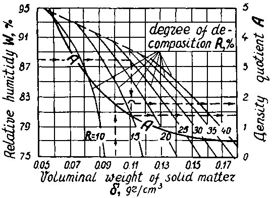
Since it is difficult to define the weight of solid matter of an undrained layer under production conditions, it is possible to choose values of A by means of the value of natural humidity, W, and the degree of decomposition, R. Determination of W and R is made by selecting samples with disturbed structure through the whole peat thickness. The nomogram (Fig. 38) also shows the method of defining the quotient A by these factors.