![]()
![]()
![]()
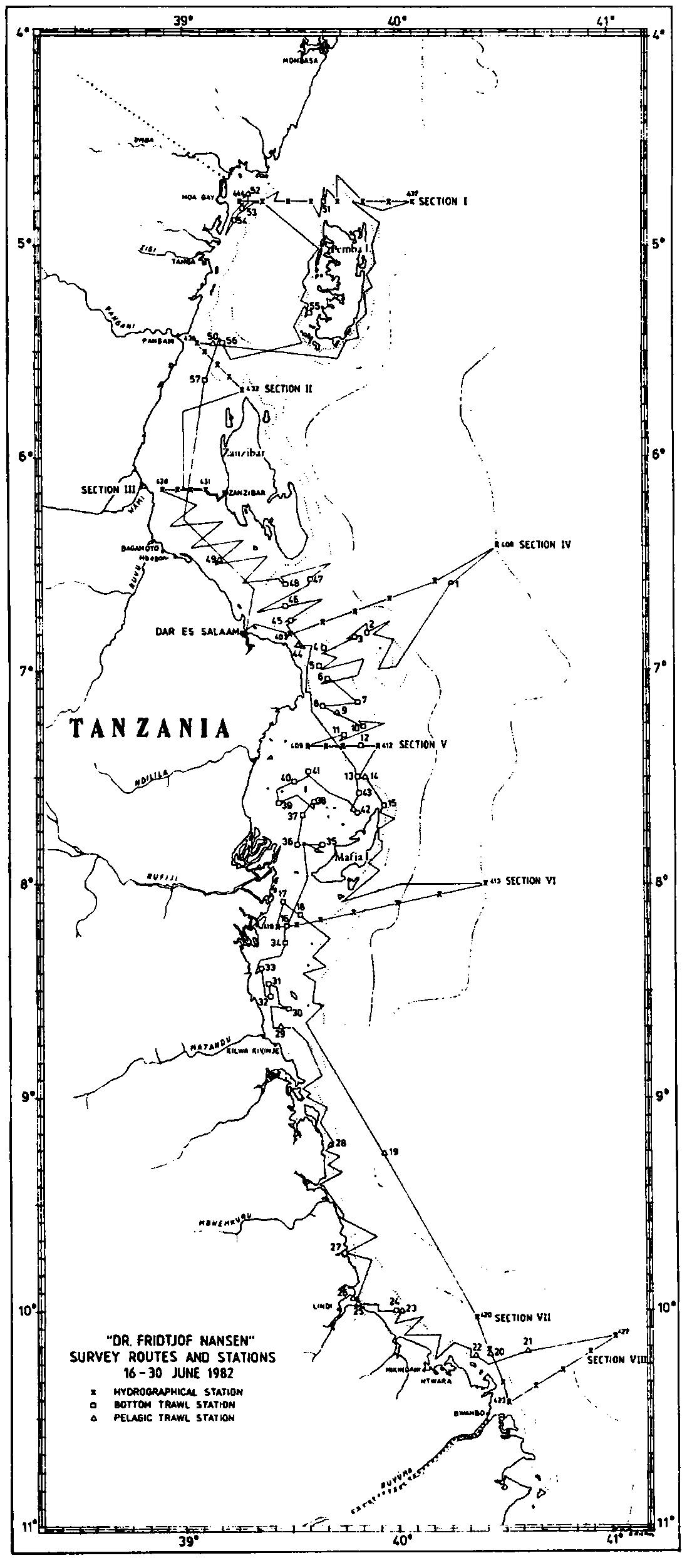
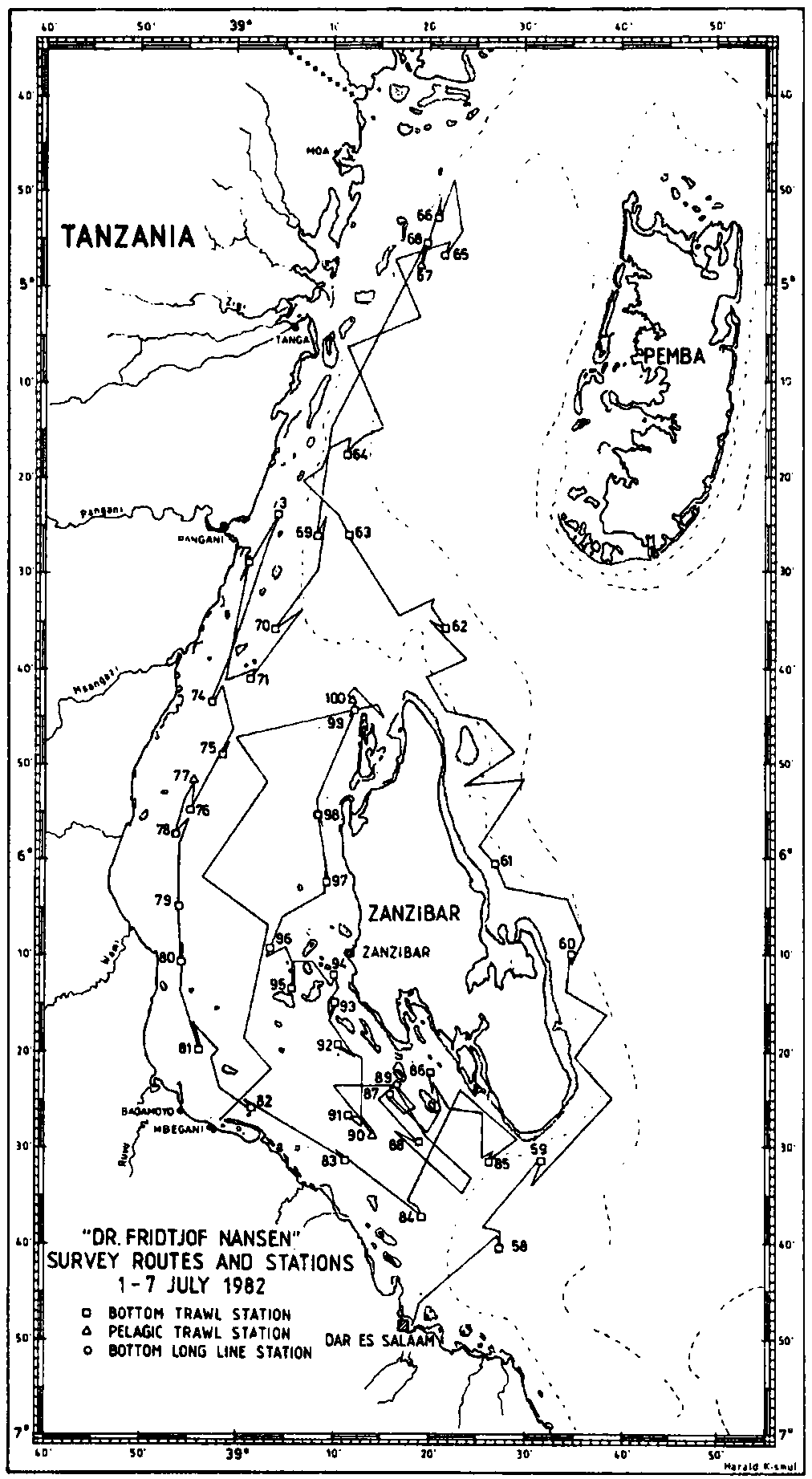
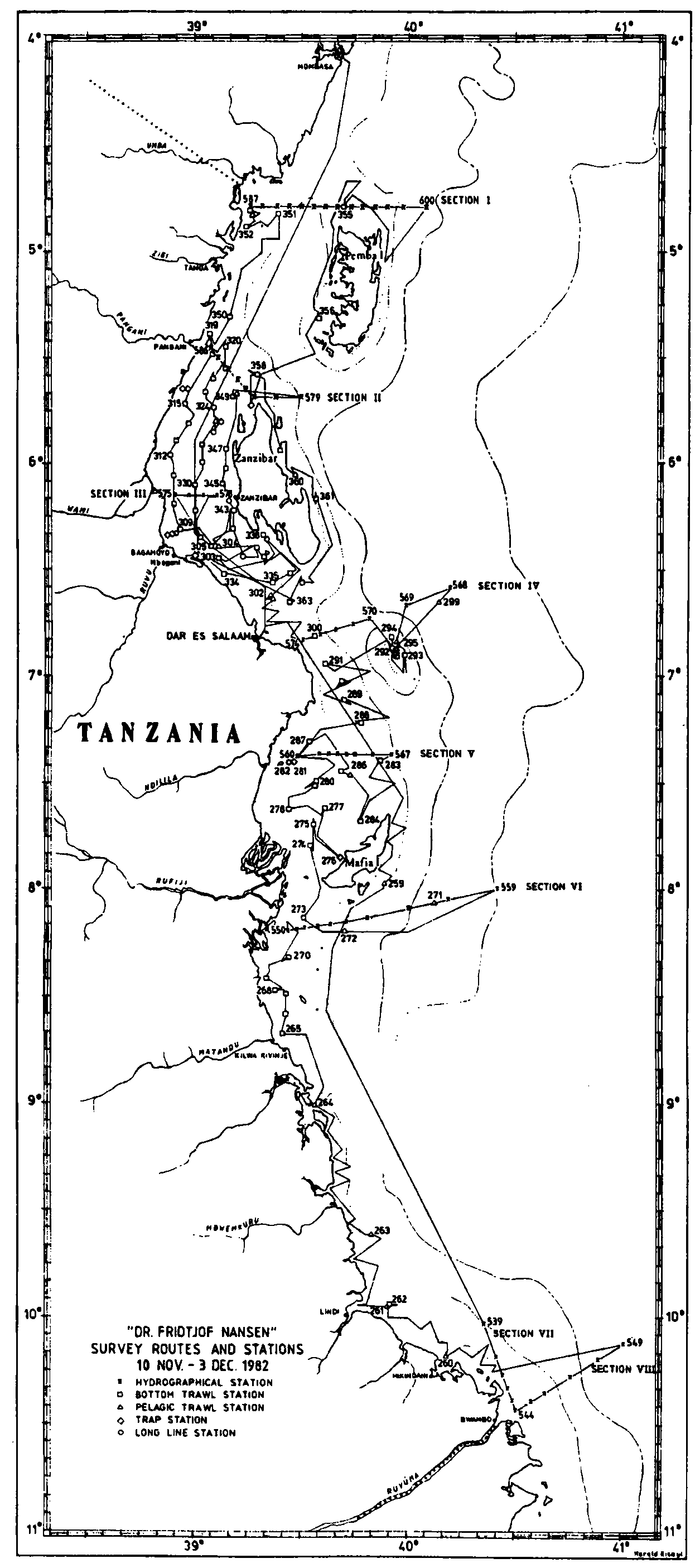
As shown in Table L1 three surveys were carried out along the Tanzanian coast with the R/V “Dr. Fridtjof Nansen” during 1982 and 1983. Two surveys in 1982 covered the total coast, while the survey in May 1983 covered the area north of Kilva Kiwinje. The survey courses, hydrographical and fishing stations for each of the surveys are shown in Figs. 2.1-2.4. During the first survey the Pemba and Zanzibar channel was covered twice (Figs. 2.1 and 2.2). During the first time the area was covered for hydrographical and acoustical purposes. During the second survey a lot of trawl hauls were carried out in the Pemba and Zanzibar channel and on the east coast of Zanzibar.
For collecting hydrographical data as temperature, salinity and oxygen content, reversible Nansen water bottles were applied in the depths 5, 10, 20, 30, 50, 75, 100, 125, 150, 200, 250, 300, 400 and 500 m. Samples from the surface were collected by a bucket. During the first survey (Fig. 2.1) eight hydrographical sections were carried out. These sections were repeated during the second survey (Fig. 2.3). During the third survey three of the sections were repeated (Fig. 2.4), and a rather dense net of stations for observing temperature and salinity in the surface was added.
The R/V “Dr. Fridtjof Nansen” is equipped for acoustic investigations of fish abundance. The vessel has three scientific sounders (120, 50 and 38 kHz), two integrators, one sonar and one net sonde (50 kHz). Each of the integrators has two channels. One of the integrators was connected to the 38 dKz sounder with the two channels operating in 4-50 m and 50-250 m. The other integrator operated together with the 120 kHz sounder in the two depth intervals 4-50 m and 50-100 m varying with depth. Echo integrator values were read as nun deflection for each nautical mile and averaged every five nautical miles. These readings were scrutinized once a day. Integrator values from false bottom and those caused by non biological targets were deleted. The integrator readings were divided into the categories: plankton/fish larvae, mesopelagic fish, pelagic fish and demersal fish. In the shallower areas the two latter categories were difficult to separate, therefore readings were assigned to the category “fish”. Average values for the fish readings were calculated within rectangles of 30 x 15 nautical miles.
Fig. 2.1. Survey routes and stations during the first part of the first survey (16-30 Jun 1982).
Fig. 2.2. Survey routes and stations during the second part of the first survey (1-8 Jul 1982).
Fig. 2.3. Survey routes and stations during the second survey.
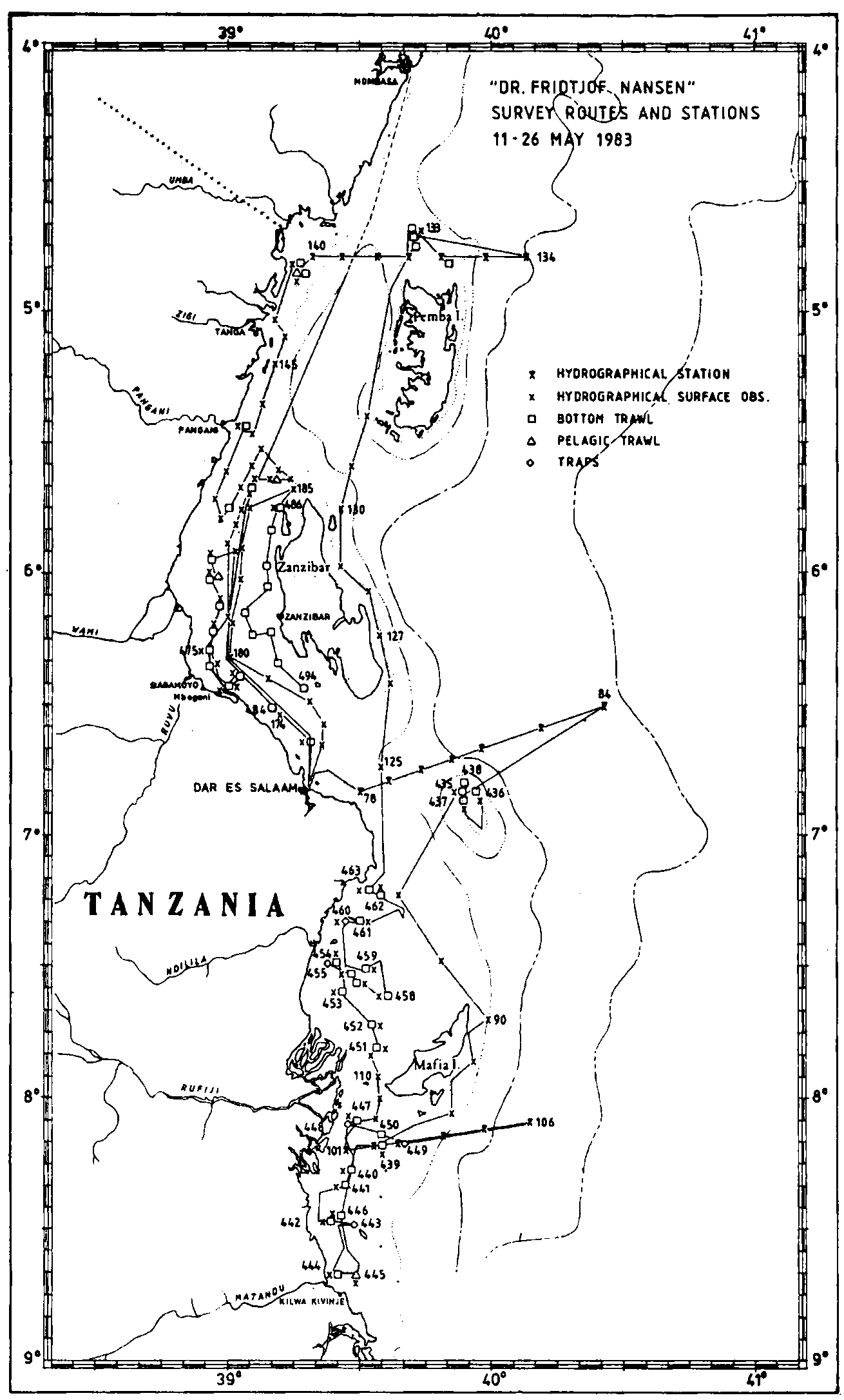
Fig. 2.4. Survey routes and stations during the third survey.
The R/V “Dr. Fridtjof Nansen” is equipped with a demersal trawl and a pelagic trawl. The specifications of the trawls are shown in Table 2.1. Pelagic trawl hauls were carried out either to identify scattering layers or to investigate the surface layer for fish. The net sonde was connected to the pelagic trawl to control that the correct depth was sampled. However, rather few pelagic trawl hauls were carried out, because pelagic scattering layers of fish were scarce and poor.
Table 2.1 Specifications of the trawls.
|
Demersal trawl: |
High opening shrimp and fish trawl with rubber
bobbins. |
|
Pelagic trawl: |
Capelin (“Harstad”) trawl. |
The most important species were measured by length and weight.
Small species were measured to the nearest 0.5 cm below, while larger species were measured to the nearest 1 cm below.
During the second survey four trawl stations were worked both by the Mbegani training fishing vessel “Mafunzo” and “Dr. Fridtjof Nansen”. These trawl hauls were made in the western part of the Zanzibar channel (Trawl stations 312-315, Fig. 2.3) in the depth region 19-45 m. “Mafunzo” is equipped with a North Sea “Calypso” trawl made in Norway. The opening of this trawl is about 2.5 times that of the “Dr. Fridtjof Nansen” trawl.
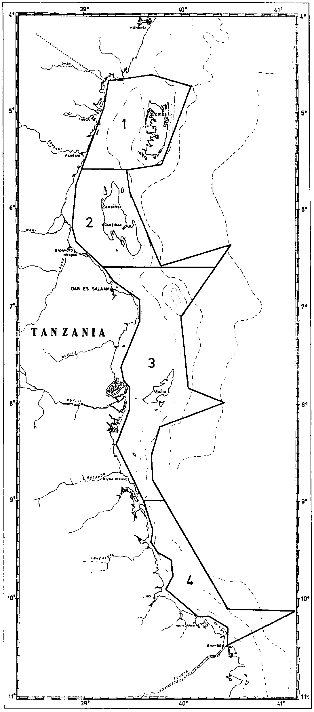
Fig. 2.5. The investigated areas:
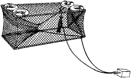
1) PembaIn selected areas longlines and special fish traps were used (Figs. 2.1 - 2.4). The fish trap which is collapsible, consists of two aluminium frames (130 x 45 cm) floats and net. The traps were usually used in chains of five. Fig. 2.6 shows a fish trap floating and expanded due to the floats attached to the upper frame.
2) Zanzibar
3) Mafia
4) The Southern area
Fig. 2.6. The collapsible fish trap.
![]()
![]()
![]()