1. Conduct of the Survey

1.1 Narrative
1.2 Plan, Equipment and Methods
1.3 Execution of the Work
1.4 Treatment of Data

1.1 Narrative

In general, the survey was carried out according to plan and without untoward event, save for an unexpected call into Muscat, on 27-30 May 1976, as a result of which the coverage of Masira Bay was relatively poor on that cruise, and for a damaged purse seine net. The SW Monsoon persisted along the Somali coast at the end of August and beginning of September, 1975 (Cruise 3), with winds reaching force 8-9 beaufort, and to a certain degree prevented fishing operations. During Cruise 5, in June 1976, the onset of the SW Monsoon, with windforce 5-6 beaufort, again to some extent prevented fishing and reliable echo integration, off Pakistan and Iran.

In early March 1975 (Cruise 1) the vessel was adrift south of Socotra while the entire crew was engaged in repairing the purse seine which had been damaged in a set some days earlier. During Cruise 2 the vessel spent 8 days, in May, at Dubai for repair of the satellite navigation system.

In Cruise 3, the plankton samples in the Gulf of Oman and off the Pakistan coast were taken with a 20 cm Bongo net, because the 60 cm diameter Bongo net had been lost off the Oman coast.

Upon completion of Cruise 2, and in the course of a voyage to Mombasa, the vessel called in at Cochin for intercalibration of its acoustic equipment with the equipment of R/V "Rastrelliger". This work provided basic date for setting a value for the conversion constant, C. During Cruise 3, on 14-15 November, 1975, the acoustic equipment of the research vessel was intercalibrated with the equipment of the Japanese research vessel "Shoyo-Moru".

After Cruise 3 the density of the survey grid was varied in accordance with the results of previous cruises, so as to give best coverage of those areas in which important resources had been located.

1.2 Plan, Equipment and Methods

Plan

The work was executed generally in accordance with the plan submitted to FAO. In 1972 in which the survey was conceived as a systematic programme of cruise in which the region would be traversed twice in each year. Essentially the work was to be an acoustic survey supplemented by fishing operations for the identification of acoustically observed organisms and for the collection of material for biological analysis, and by oceanographic work (hydrographic stations and plankton collections) by which to make an ecological characterization of each part of the surveyed region.

In the work-plan it was assumed that "the off-shore extent of the survey will be limited to abt. 300 nautical miles" but in the event most of the work was carried out in a coastal zone of which the average width was about 12.5 nm. Moreover, the easterly limit to the survey was set at the Pakistan/India border, thus excluding the coast of India. With this reduction of the total area to be surveyed it was possible to carry out the work with one vessel, rather than with two as contemplated in the work-plan.

Vessel and gear

The R/V "Dr. Fridtjof Nansen" is 150 feet long, a combined stern trawler and purse seiner. A main engine of 1500 horsepower gives a maximum speed of 13 knots. There is accommodation for 28 men. All winches are hydraulic. The vessel carries two pelagic trawls, one bottom trawl and one purse seine, some gillnets, bottom lines and hand lines. Fig. 7 shows the main deck arrangement. All gears were ready for use on short notice. The details of the fishing gears are given in Fig. 8 and Fig. 9.

A satellite navigator is included in the navigation equipment, allowing very precise determination of position.

Acoustics

The acoustic equipment consists of 3 scientific sounders (129, 50 and 38 kHz), 2 echo integrators, 1 searchlight sonar (18 kHz) and 1 netsonde (50 kHz).

The two echo integrators were coupled to the 50 kHz scientific sounder, integrating the depth slices 8-50, 50-100, 100-150 or 100-250, 150-350 or 250-450 m. The settings of the sounder were as follow: Basic range: 0-100 or 0-250 m - Transmitter 10 kW - Pulselength and bandwidth 0.5 msec, 1 kHz - Receiver TVG and gain 20 logR-20 dB - Recorder gain 6 or 7. The gain on the echo integrators was mainly set to 30 dB, and the threshold setting was 1. Echo integrator values were read for each nautical mile sailed and average values for each 5 nautical mile were calculated and logged. All logged echo integrator values were referred to 30 dB gain on the integrators and the above-mentioned settings on the sounder. The 120 kHz and 40 kHz echo sounders were used for a "closer look" at interesting recordings. The sonar was operated continuously, mainly on range 0-2000 m.

Continuous watch was kept on the acoustic instruments, and fishing operations for identification purposes were carried out whenever the echo sounder recording changed its characteristics. The acoustic data were scrutinized once each day. Echoes and integrator contributions from false bottom, wakes etc. were deleted, and the integrator readings were grouped in four categories: small pelagic fish, mesopelagic fish, demersal fish, 0-group fish and plankton.

The sonar counting technique described by Smith (1971) was used in localities where small near-surface schools were found. The sonar was then used on basic range 0-500 m. The transducer was kept constantly trained at 70° to the starboard or port side, and the schools appearing on the recording paper between 100 and 500 m were counted.

Since the 10 kW transmitter for the 38 kHz echo sounder failed for a part of cruise 2, the investigations in the Gulf of Oman and parts of the coast of Pakistan during that cruise were carried out with the 1 kW transmitter and the receiver setting 20 logR - 0 dB. Later the two transmitters were intercalibrated and the following relation was found:

11.7 . M₁ = M₂

where M₁ is the integrator output using the normal setting and M₂ is the integrator output at 1 kW transmitter and 20 logR 0 dB receiver.

The vessel's acoustic equipment was calibrated with that of other vessels so that with correctly measured factors the echo-integrator output of the one could be converted to comparable values of the other. During the intercalibration run of R/V "Rastrelliger" and R/V "Dr. Fridtjof Nansen" the two vessels sailed 24 nautical miles, one closely following the other but avoiding the wake. The log counter/reset facilities on the two vessels were synchronized before start. Recordings of single fish and scattering layers were fairly good during the run.

The result of a least mean square analysis of the observed integrator outputs was:

Ras (120 kHz) = F.N. (120 kHz) 7.9 - 13
Ras (120 kHz) = F.N. ( 38 kHz) 1.1 - 11

Fish biology

The following guidelines were followed in the biological work:

A. GENERAL:

- Large fish (each specimen): Length - Weight - Sex - Maturity stage - Gonad weight - Volume of total stomach contents - Sample material for age determinations - Observations and collections of ecto- and endo-parasites.

- Small fish: Weight of entire sample - Length of each individual - Weight of each length category - Number in each length category - Five (or more) fish in each length category were examined as above - Mean weight was computed.

- Bony fish: Fork length (LF₁) measured from the tip of the snout (mouth closed) to the posterior tip of the central (shortest) caudal fin ray. Small species were measured to the 0.5 cm below the measurement and large species to 1 cm below the measurement. For Trichiurus total length (LT₁) was measured to the 1 cm below.

- Lobsters: Carapace length (CL₁) measured from the tip of the rostrum to the posterior edge of the cephalothorax.

- Crabs: Carapace width (W₁) measured across the widest point of the carapace, including spines.

The ponderal index or condition factor (K) was calculated from: where W is the mean weight for each length group. The criteria for the observation of maturity stages were as follows:

Maturity state	Stage No.
Immature	I
Mature unripe	II
Mature ripening	III
Mature nearly ripe	IV
Mature ripe (Non spawning)	V
Mature ripe running (spawning)	VI
Mature spent	VII

Stomachs were denoted full (8), about half-full (4) and empty or nearly so (2) by visual estimates.

Fatness was determined by visual observation of alimentary fat deposits as follows:

1: lean	- no trace of fat on digestive tract.
2: fattening	- fat strands few, less than about 2 mm thickness on digestive tract.
3: fat	- fat strands of more than 2 mm thickness on digestive tract but not obscuring viscera.
4: very fat	- fat deposits entirely obscuring viscera in body cavity.

Plankton

Plankton samples were taken at the hydrographic stations from oblique tows with a 60 cm diameter Bongo net of 300 mesh size. The net was lowered to 50 m depth and then hauled at a vessel speed of 1.5-2 knots. Displacement volumes of the samples were measured on board.

Hydrography

The vessel is equipped with 20 Nansen water bottles for hydrographic work. Temperature readings and seawater samples for salinity determinations were collected at hydrographic stations at standard depths: 10 - 20 - 30 - 50 - 75 - 100 - 125 - 150 - 200 - 250 - 300 - 400 - 500 m. Salinities were determined on board using an inductive salinometer. Samples for oxygen titration were taken at 10 - 30 - 50 - 100 - 150 - 200 - 250 - 300 meters and oxygen content was determined by the Winkler method. On each hydrographic station and on most of the fishing stations continuous temperature/depth curves were obtained with the bathythermograph. A thermograph recorded the temperature continuously at 4 m depth.

1.3 Execution of the Work

The region surveyed, and its divisions, are geographically described in Table 2. The total coastline is approximately 3,530 nm. The total distance travelled in the course of the survey was approximately 33,500 nm of which approximately half was devoted to the intensive survey work over the continental shelf and some immediately adjacent oceanic waters. The remainder of the mileage was devoted to special, wider-ranging oceanic traverses, especially across the Gulfs of Aden and Oman, to fishing operations and to service travel.

The total shelf area is approximately 44,000 nm². Since in some sectors, during some cruises, the acoustically-observed stocks occupied waters both over and beyond the continental shelf, the surveyed space in 7 cases in Table 3 is shown as having been of area more than 100% of the area of the shelf; substracting the "extra" areas from the total surveyed area (Col. 9 of Table 3) leaves a total of 32,384 nm² which constitutes 73.6% of the area of the shelf.

In order to avoid ambiguities in reporting the analysis of survey results it is necessary to name and define a number of different kinds of "areas", but in the first place we must point out that we endeavour (and hope to have succeeded) to avoid using the word "area" other than in the specific sense of "superficial extent", as in "the area of the continental shelf of Sector 1 is 9,340 nm²".

By "sector" we refer to a defined part of the ocean space over which the vessel moved in the course of this survey; we have defined 7 such sectors in Table 2. Each sector comprises continental shelf space and oceanic space, the division between which is marked by the 100 fm contour. The total area surveyed is thus the number of square nautical miles of ocean space over which the vessel moved whilst survey work was being done; it includes a considerable amount of oceanic space of which it is difficult to measure the area. The area of the continental shelf can be measured by virtue of the bounding lines (coast, 100-fathom and the inter-sectorial lines drawn for the survey), and Insofar as the vessel traversed the whole or part of this space, the survey area can easily be measured, and the density of survey can be given; in the case of oceanic survey however, determination of the distance on each side of the vessel's track to which its observations can be held to be representative presents some difficulty, thus "total area surveyed" must be a somewhat uncertain figure.

This report, however, relates mainly to work over the continental shelf the space of which has been marked, variously into 3 types: "patches", occupied space and unoccupied space; the first of these terms refers to the individual pieces of shelf space in which positive recordings were made and which are marked off by estimator boundary lines as in Figures 10-21; the sum of the areas of these patches within a sector, as observed in the course of a cruise, is the occupied space of the sector; the difference between the area of the continental shelf of a sector and the observed occupied space is unoccupied space in which only zero recordings have been made.

In the acoustic work, 3.9 recordings* were made per 100 nm², on the average over all cruises; this signifies 19.5 nm of acoustic track per 10-mile square, which in turn signifies that each unit area was traversed twice on each cruise. The intensity of survey, as measured by this index, varied from cruise to cruise, being greatest on the first two cruises (4.1) and least on Cruise 5 (2.5). The intensity varied also between sectors during each cruise the variation being greatest on Cruises 1 & 2 (the greatest intensity being nearly 4 times the least) and smallest on Cruise 3 (with ratio less than 2). More detailed information on survey intensity is to be found in Table 3.

* The word "recording" is hereafter used, throughout the text, to signify the 5-mile-average integrator recording.

Oceanographic stations were occupied on 939 occasions and 225 plankton sample were taken.

From this summary, and the relevant tables, it will be seen that the survey work was carried out duly according to plan. A basis for an evaluation of the work of this survey can be found in data from acoustic survey work in the Barents Sea in which the number of recordings per 100 nm² was 8.7 in 1977 and 8 in 1978. Considering that the Barents Sea work was directed upon a well defined region and stocks of which much is known, in contrast with the exploratory nature of the work in the Arabian Sea, and considering the greater size of the vessel with which the Barents Sea work was carried out as well as operational differences in the work of the two area, the survey intensity of 3.9 recordings per 100 nm² obtained with R/V "Dr. Fridtjof Nansen" must be regarded as quite satisfactory.

1.4 Treatment of Data

The data with regard to fishes taken in the catches were treated, in the first instance, by the usual biological methods, of presentation in histograms and calculation of mean length (and its standard deviation) and mean weight. Species-composition tables, by cruise and by area, were also prepared.

For the estimation of the conversion constant, C, mean length of the acoustically observed fishes had to be calculated; this was done by the following procedure. A record having been made of the number of individuals of each species in each catch, and of their total weight, the mean weight of the captured individuals of each species could be calculated. A corresponding mean length was then calculated from the formula:

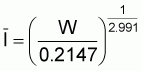
This formula is derived from the familiar weight/length relation W = aL^b with values of the constants for Caranx carangus given by Franqueville and Freon (1976). This species was chosen, from among 28 species for which Franqueville and Freon give W/L formulae, as an "average fish". Thus, values of and N (number of captured individuals) were available for each species in each catch. A length frequency table, of 20 size-classes, was then prepared for each sector by assigning the number of individuals of each species of each catch to the size-class corresponding to the of those individuals. A sector mean length of all species was then calculated from this table.

In the preliminary final report the recordings were averaged for each 1° square and biomass was estimated from these mean values. This treatment, however, made Inadequate and perhaps inaccurate use of the information obtained during the survey: it abandoned the measure of variation in the data, and blurred the indications of distributional patterns. An alternative treatment was therefore applied.

The recordings, separately of demersal and pelagic fishes, were written onto maps on which the survey track had been traced. The two values at each observation point were added and "contour" lines were drawn, by eye, around groups of values of more or less the same magnitude. These groups constituted patches whose area could be measured by planimeter and for which mean and variance could be calculated. The patches were then classified in strata, with mean values from 0 to 9.9 (I), from 10 to 29.9 (II) and greater than 30 (III). For each sector a mean and variance was calculated for each stratum, for demersal and pelagic separately and for the sum of the two; overall sector means and variances were then obtained by weighting the stratum values by the area of the "patches" of each stratum. Confidence limits were then calculated and these became the values from which an estimate of biomass, demersal and pelagic, was to be made. Each value was then multiplied by the area of the sector to which it related to give a sector total integrator value, and the final step was to multiply each such value by an appropriate value of the conversion constant, C.

A value of the constant C (weight of the biomass of 1 square nautical mile that gives an integrator value of 1 mm; see, for example Forbes and Nakken, 19 ) had been obtained from the inter-calibration work with the R/V "Rastrelliger". This value was 10 t/nm² for a fish of length 17 cm. Since experimental work (see, for example, Nakken and 01 sen) had shown that for a particular species the value of C is directly proportional to length, it was assumed that as a first approximation the value of C for a sector could be calculated from the formula:

in which is the mean length of the fishes present in the area in which the integrator recording had been obtained. A mean value for length of all fishes of Interest in each of the sectors was obtained as described above.

The central and largest body of data is the set of echo-integrator recordings As described above, these were scruitinzed once each day; the scrutiny was a team consultation during which, after deletion of non-biotic contributions, the recordings were grouped and partitioned into the four categories of biota the data with which this report is concerned are the values assigned to the categories small pelagic and demersal. The grouping and partitioning was effected by reference to evidence available in the characteristics of the echo-traces, and to other evidence from fishing and from surface observations; it was subject to arbitrary criteria as to the category to which each species or kind of fish or other biota was to be assigned and to the ability of the observer to associate particular kinds of traces with particular species or kinds. Of course, the critical confirmatory evidence was to have come from fishing, but if, at any time and for whatever reason, this were inadequate the identification and hence the grouping and partitioning would be faulty. This indeed was the case with the work in the Gulf of Oman during the final cruise; the recordings on that occasion were identified as caused by small pelagic fish, but subsequent examination of the traces and recordings indicated that the bulk of the acoustically observed biomass was of mesopelagic fishes, they do not however provide evidence from which to decide upon the fraction of the recordings that should have been assigned to small pelagic fishes which, undoubtedly, must have been present in some quantity; for this reason all the readings in the Gulf of Oman of Cruise 5 have been abandoned. For a different reason, namely change of criterion, another block of data, from the southern part of Sector 1 (off the Somali Coast), obtained during Cruise 4, has been abandoned. In that case some large concentrations of Synagrops, correctly Identified, were assigned to the small pelagic category since at that time that genus was held to be small pelagic; subsequent evidence led to Synagrops being counted as mesopelagic but by that time it was too late to make a revised assignment to small pelagic.