3. Survey Results

3.1 Composition of the Catches
3.2 The Acoustic Measurement of Biomass
3.3 Bionomic Aspects
3.4 Catch Rates and Fishing Prospects
3.5 Environmental Information

3.1 Composition of the Catches

The basic rule for deciding when and where to fish, laid down in the adopted work-plan, was that fishing should take place whenever the character of the echo-trace changed. Thus, theoretically, all traces, except those from the beginning of the cruise until the first catch, should be catch-identified, and it should be reasonable to assume that all integrator readings recorded after one catch and until the next catch were a measure of the biomass of stocks of the composition revealed by the first catch. The basic rule implies, however, that each significant change in stock composition will be clearly manifest in the echo-trace and readily detectable by a trained observer; but if, as is most probable, stocks of different species can cause echo-traces indistinguishable from one another, the basic rule is inadequate. Adding to this the humanly inevitable failure of observers at times, from fatigue or for other reasons, to detect or to react to changes in echo-traces then it must be accepted that catches taken in obedience to this rule cannot provide comprehensive and accurate evidence of the composition of the observe stocks. Again, the rule may be sufficient if the criterion of significance is that the change in character should be only such as to require a change of conversion factor and if the objective of the acoustic work is solely to measure biomass, irrespective of composition of the stocks. But if the composition of the stocks is of importance, as indeed it was in this survey the rule is still more inadequate. On the other hand, it is to be borne in mind that the catches were not the sole source of evidence of stock composition: other information is available from the records of surface observations, such as of schooling behaviour. This other information has, of course, been taken into account in the analysis of acoustic records.

The survey objectives with regard to stock composition extended beyond specie identification to include, as the work-plan required (see Section 1.2), observations of length, weight, sex, sexual condition and stomach contents, and samples of catches were taken for this purpose. However, in this respect too the results are inadequate: the number of fully analysed catch samples is relatively small and it is for this reason that mean length of individuals of observed stocks (for determination of the value of the conversion constant) had to be made in the manner described in Section 1.4. Table 4a shows, for each sector, the number of species which appeared in the catches of only 1 cruise, those that appeared on 2 cruises and so on. Similarly, Table 5a shows for each cruise the number of species which appeared in all 5 sectors, those that appeared in 4 sectors and so on. It will be observed that in the two tables the distributions are notably similar; in Table 4a, the means for two sectors fall outside (one below and one above) the 95% confidence limits of a weighted mean for the whole table. The data of these tables are combined in Table 6 where, the concentration in the upper left-hand sector of the table is considerable; few species (3%) occurred in all 7 sectors in all five cruises, and most species occurred in 1 or 2 cruises (67%) in 1 or 2 sectors (53%). Table 4a is to be interpreted as giving some Indication of seasonal variability of the accessibility and vulnerability of the species of which the biota is composed; Table 5a, on the other hand, gives an Indication of ubiquity compounded with the indication of variability of accessibility and vulnerability. In addition, the results in these tables to some degree reflect simply the chanciness of the particular fishing operations by which the samples were obtained.

A result somewhat the same as that of Table 5a is presented by tabulations of

(a) appearances of families in the catches (Table 7a);
(b) citation, in the text of the cruise reports, of species observed (Table 7b), and was obtained by Druzhinin (1973), as the following figures show:

But in Table 7a there is evidence of another aspect of this matter. Not only are the appearances low -- in pelagic fishing each family appeared on the average in only 3% of the hauls whilst in demersal fishing each family appeared in 12% of the hauls -- but of the 55 families, 39 appeared in both pelagic and bottom trawls while only 2 families appeared in only pelagic haul and 14 families appeared only in bottom trawls. It is yet to be ascertained whether what holds for these 39 families, that is, that they can be caught both in surface and bottom waters, holds as well for the species of which they are composed, or that in each family some species are pelagic and some demersal. Nevertheless, the evidence here throws some doubt on the validity of the distinction between pelagic and demersal types. The considerations here depend largely on the definition of pelagic and demersal fish and on the way the trawls are operated. Often, particularly in shallow waters, the pelagic trawl was hauled on or very close to(1/2m) the bottom.

Druzhinin (1973) in a report on similar work relating to a large part of the region to which the present report relates, listed some 322 species taken in fishing operations. For the present survey a list of 456 species and 128 families was drawn up and coded. The family codes (as distinct from species codes) are many times entered in the catch records with report of quantity taken. In some cases such records related to species for which codes existed but final species identification was not made; in other cases a record of family code related to specimens that could be assigned to the family but which were not of the recognised and coded species. Thus the total number of species was not less than 456 and might have been as many as 584 (456 + 128) or even more. Table 8 presents a summary of data on the number of species found in each shot, of surface pelagic net, of bottom trawl and other gears, and by all gears. The geometric mean number of species in a shot, for all gears, is 7.4 which means, supposing that species were caught entirely at random and that once a species was taken in the course of a cruise it would not be taken again during that cruise, that for 584 species a minimum of 79 shots would be required to obtain specimens of all species; but, since on the average, each species made about 2 appearances in the course of a cruise, a minimum of 158 shots would be necessary under these unrealistic conditions. If then we modify our specification of conditions, and we make them more realistic by, on the one hand, reducing the chance that a gear will take specimens from all species present in a locality at the time of a shot, and, on the other hand, reducing the fit of the distribution, abundance and behaviour of each species to the distribution in time and space of the fishing operations, the required number of shots is considerably greater. The original, unrealistic conditions imply a value of 1 for the gear catching-power ('catchability' of authors) whereas a value of 0.5 would probably be more realistic*. Those conditions also imply that every species is present within each sector in one or other of the fished localities at the times of fishing, represented by individuals of a size and abundance that would make it likely that a gear with catching-power of 0.5 would take some specimens of it. This condition, however, is highly improbable: some species are of such limited distribution and their numbers so small that they are taken only extremely rarely, even by intensive fishing of a locality; the pattern of distribution of some species is so changeable that their presence in some locality might never synchronise with fishing operations there; species of short life-span may be represented at times by only post-larvae are small juveniles. Theoretically, each species could be rated, as to its availability/accessibility/vulnerability (AAV index) to a specified net, on a scale from 0 to 1; a species which is always present, abundant and catchable would be rated 1, others, such as those just cited, would be rated less. The average rating might perhaps be 0.5 and if that were the case the number of shots required, taking also into account the fishing-power factor of 0.5, would be 632 per cruise 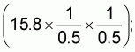in contrast, the average number of shots per cruise (counting the first two cruises as one) was 90.

* We hold that catchability holds as much between species as it does between size-groups of a species, especially since each species is characterized by a mean size.

3.2 The Acoustic Measurement of Biomass

The raw data from the acoustic work are the recordings, summarised in Tables 10a to g, and as a first step, we must examine the statistical characteristic of these data. It will be seen in these tables that the variances without exception are greater than the mean and generally are many times greater.

Thus it is clear that the observations were of contagiously distributed populations, a feature which was already obvious in the patchiness shown in Figures 10 to 21. Moreover, a strong correlation holds between mean and variance, as exemplified by Figure 22; the data from which this figure was drawn are the means and variances for cruise and resource type (demersal and pelagic) of Sector 1 in Table 9a. Similar results, with even higher correlations, were obtained for other Sectors, and for patches and strata but with lower correlations. Roughly the result is:

Value of Mean	Value of Variance
< 10	about 7
10 £ < 30	15
> 30	60

The effect of this characteristic is that some statistical methods "including the t-test and analysis of variance, cannot be applied without the risk of considerable errors" (Elliott, 1977). The appropriate course of action, in this situation, would be to transform all the data, replacing x by log (x + 1) (Elliott l.c.); unfortunately the complete set of original data was not readily accessible at the time of preparation of this report and therefore the analysis has been made at the simple level of arithmetic means and variances, leaving until some later opportunity such deeper analyses and more subtle comparisons as might be made with transformed data.

The mean sector/cruise recordings are assembled in Tables 11a and b for ease of comparison. The distribution of these values is, in both cases, highly skewed positively and highly leptokurtic but after transformation (replacing x by log (x + 1) each distribution is close to normal. The values for demersal stocks are relatively uniform in two blocks, Sectors 1 and 2 and Sectors 3 to 7; also there is some grouping between cruises: Cruise 4, which was executed entirely during the NE Monsoon, has lowest mean, Cruises 1/2 and 5, whose execution extended from the end of the NE Monsoon through the transitional month April into the beginning of the SW Monsoon have the same mean, while the means of Cruises 3 and 6 (with converse location in time, from end of SW Monsoon through October into the beginning of the NE Monsoon) are almost the same and are higher than the other two. Analysis of variance of these transformed means results in F-test value at 5% for comparison of the cruises mean square with residual mean square and at between 5% and 1% for comparison between sectors and residuals. The coefficient of variation (of transformed values) for pelagic (40.5%) is only little more than that for demersal (38.7%), and although analysis of variance shows comparisons in Table 11b are non-significant, they are not without interest. As in Table 11a, there is a grouping of the sectors, Sectors 2 and 5 being highest, Sectors 1 and 2 being next (and these two pairs are nearly equal), and Sectors 3, 6 and 7 are substantially lower than the others. The Cruise 4 overall mean is in this case the highest and those of Cruise 1/2 and 5 are lowest (but not equal) whereas those of Cruises 3 and 5 are equal. This suggests that comparisons between cruises might not be correct and that these values should instead be grouped by seasons (see Figure ); when this is done still greater differences appear for pelagic: the overall mean for values obtained in the NE Monsoon is 11.6, for the SW Monsoon is 6.4, April 3.9 and October 7.9. For demersal stocks the effect of this regrouping is the opposite, the coefficient of variation of the seasonal values is half that of the cruise values. Thus, it may be taken that, despite having some species in common, the demersal and pelagic biota show marked differences of acoustic density both spatially (between-sector differences) and temporarily (of difference of seasonal response); but there are indications, even in this analysis, of sector/season interactions for which we have not yet made any allowance.

It is to be kept in mind that the data in Table 10 are simply mean values of recordings each of which has the same weight as every other; they therefore are merely indices of acoustic density. The sets of these values, relating to separate patches, grouped in strata, must be weighted each according to the total area of the patches of the stratum to which it refers. This analysis has shown, however, an approach to the analysis of the weighted and converted data which we take to constitute measurements of biomass.

The biomass estimates are made from the stratum-area weighted mean recordings for each sector during each cruise; the successive calculation steps are set out in Table 11, and it will be seen that the confidence limits of each mean have been calculated.

The sector/cruise biomass estimates are set out in Table 12 a and b. Interpretation of these values, with overall range from 3,000 to 1,087,000 tonnes and considerable differences between cruises and between sectors, is somewhat difficult, because, in the first place, of differences of area of the sectors, and, in the second place, of the problems of seasonality discussed above. To reduce the area effects the figures have been converted in Table 13 a and b, to biomass per square mile of continental shelf; these values have an overall mean of 36.1 t/nm² for pelagic and of 17.4 t/nm² for demersal the sum of which gives about 17t/km² which is similar to estimates made for other regions of the northern Indian Ocean (Raja, 1980). In the table of pelagic values, the low figures for Sectors 6 and 7 may have resulted from the absence of data from the last cruise, otherwise the Gulf of Oman appears to be less productive of pelagic stocks than are the other sectors.

But, while this conversion of the biomass estimates adds some confidence to inter-sectorial comparisons, some doubts remain as to what in fact is being compared and what the estimates are of: are the individual cruise values truly representative of the amount of biomass of some period? and, if so, of what period in each case? among the individual values, is the greatest a measure of the maximum reached by the stocks? and are the mean values a true measure of the average to be expected in each sector, or do they measure that to which authors refer with the expression "standing stock?"

In the first approach to this analysis we assumed that the biomass of each stock must fluctuate each year and we further assumed, with regard to the acoustically observable stocks, that the fluctuation must be from a minimum at some time shortly after spawning, when the mature individuals had lost weight from spawning and replenishment of their numbers by recruitment had not yet overtaken the loss by natural mortality, to a maximum produced by recruitment and the rapid growth of the recruits. We also expected, though with less confidence, that the maxima (and, therefore, also the minima) would occur in the same season for such a proportion of the stocks that a similar annual cycle would appear in the total biomass. Although the recordings indicate, as discussed earlier in this section, that the pelagic stocks are at their maximum during the NE Monsoon and at their minima in the transition month April, Figures 23 a to g give meagre support to our assumptions, and chiefly in the case of Sector 2 in which both demersal and pelagic stocks show something like an annual cycle.*

* The individual curves in these figures are discussed in greater detail below.

However, the evidence, although it gives only weak support to our assumptions does not point to a rejection of those assumptions and even less does it suggest alternative assumptions. We return to these questions after the following examination of evidence with regard to each of the seven sectors, in turn.

Sector 1 Somali east coast 2°N 46°E to 11°N 51°E*

* These indications are only approximate.

Round herring (Etrumeus teres) was found in relatively small quantities in the southern part of this sector during most of the cruises. During April 1976 (Cruise 5) this species was observed in small schools and scattering layers a depths between 50 and 100 m and at depths of 120-160 m just off Mogadiscio. The recordings of round herring, sardinella (Sardinella sp.) and spotted herring (Herklotsichthys sp.) were not so dense as to promise commercial catches with the gears used by "Dr. Fridtjof Nansen".

The most important pelagic fish species observed in the northern part of the sector was the mackerel (Scomber sp.), which was observed along the edge of the continental shelf between 5° and 8° N during spring both in 1975 and in 1976. During the day the fish formed small schools at the bottom at 300-350 m depth while during the night they appeared as a pelagic scattering layer in 150-200 m depth.

In November 1976 (Cruise 6) several schools were recorded near the bottom at depth of 150 m in the area of Mogadiscio. These schools were classified as mackerel but the true identity could not be established because trawling conditions were unsuitable. If these recordings originated from mackerel, the observation may serve as an indication of a seasonal shift of concentration since it was made 180-300 nautical miles south of the area where the fish was observed during the spring cruises.

Scattered recordings of anchovy (Engraulis sp. and Stolephorus sp.) and scad (Decapterus sp.) were observed in nearshore waters during all cruises.

Relatively high abundances of small pelagic fish were observed in the northern-most part of this sector during all cruises except for Cruise No. 4. The recordings originated from Indian oil sardinella (Sardinella longiceps), round herring and scad (Decapterus macrosoma and Decapterus maruadsi). The fish was observed in near-surface schools and in scattering layers at 10-30 m depth over the shelf area between Ras Asir and Ras Hafun. The observations indicate both higher biomass and higher availability of the fish for fishing operations in autumn than in spring. During the spring surveys the schools were observed to be small while schools of more than 100 tonnes were found in autumn 1975.

Near-surface schools were only partly recorded by the echosounder, and therefore their biomass was estimated from sonar counts of the schools; during the spring surveys their biomass amounted to only a small fraction of the total pelagic biomass, but in autumn 1976 (Cruise 6) it was found that schools of this kind within the area constituted about 1/6th of the total.

The observations on the state of the gonads of the small pelagic fish caught in this north-eastern locality are especially interesting, and are of particular relevance to a consideration of the AAV Index in connection with a possible annual cycle of fluctuation in biomass. Indian oil sardinella and layang scad were observed to be mainly ripening and nearly ripe, during all periods of observation, with higher percentages of nearly ripe during the autumn surveys. A significant portion of the Indian oil sardinella stock was spawning in November 1976. The round herring was ripening during the spring surveys while the fish observed in October 1975 were recently spent, the fish of small size observed in November 1976 were all immature. These observations indicate that the area is a spawning locality for all three species. The observations show that the Indian oil Sardinella and probably also the layang scad spawn in late autumn while the round herring spawns earlier in the autumn. The observations of ripening stages in early spring indicate also a spawning period for all three species in late spring. This evidence is referred to again in the section below relating to Sector 3.

The maximum biomass density in January, shown in Figure 23a1, is perhaps consistent, within our assumptions, with the evidence of autumn (?September) spawning, and so then also might be the low value in August, but the minimum in February of 1975 can scarcely be accepted as a true measure of the sector pelagic biomass during the NE Monsoon; but, by the same token the value for October 1976 does not correspond well to the October 1975 value. Thus, if we accept the central three values (August, January and April) we must hesitate about accepting the first and last values, or if we accept the latter we must doubt the former. Short of attributing this situation to technical errors in operation and reading of equipment and/or in the analytical procedures, we are bound to make further assumptions to the effect:

(a) that the stocks tend to form in localised concentrations

(b) that the concentrations shift about within a sector, and perhaps at times move out of it; and

(c) that in the course of a cruise the observations might happen to be consistently of unoccupied space.

(d) that year to year variations in stock sizes occur.

Demersal Fishes:

A large amount of demersal stock was observed in the northern part of this sector in autumn 1975 (Cruise 3) but was not identified. The recordings were made at depths between 100 and 300m in the locality in which mackerel had been observed in spring (Cruise 1/2), but since bad weather conditions created a lot of noise on the echosounder no conclusions could be drawn as to the origin of the recordings and since such density was not observed in that locality during later cruises we can do no more than note the observation.

Mention must be made here, with relevance as well to results relating to demersal stocks of all other sectors, to the fact that the echosounder had a dead zone in the bottom 1-2 m of water depending on depth and bottom configuration, failing to measure biomass lying in the bottom 3m of water. All estimates of demersal biomass density are therefore subject to the possibility that significant quantities of biomass lay, unmeasured in that bottom stratum. Since there is good reason to suppose (a) that whenever demersal stocks are observed in a locality some proportion of them lies in the bottom stratum, (b) that in some times of the day and in some seasons the concentration in the bottom stratum is very high, and (c) that in some localities in which the echosounder gives no indication of the presence of demersal stocks there might nevertheless be some stocks in the bottom stratum, it may also be supposed that all values of demersal biomass density obtained during the survey are lower than the true values, except where other causes (see p. 38) have resulted in an overestimate of what has been observed. In balance, however, we believe that the demersal stock, in general, has been underestimated.

The two maxima of the curve, in Figure 23a2, for demersal stocks of this sector at first sight seem to conform to the assumption of an annual cycle but they differ importantly in timing; therefore, except in the event that a 3-month shift had taken place of one or the other, one of these cannot be a measure of the maximum reached in its year. Graphically, as suggested by the dashed line on the left of the figure, it seems plausible to suggest that a maximum had been reached in April 1975 when, however, the vessel was elsewhere.

Total Biomass:

From the evidence available we conclude that the pelagic biomass of this region can reach a maximum of 116 ± 14 t/nm² and the demersal biomass a maximum of 65 ± 23 t/nm² which means in total, with continental shelf area of 9,340 nm, from about 953,000 to 1,214,000 tonnes of pelagic biomass and from 392,000 to 822,000 tonnes of demersal biomass. Since the maxima of the two types do not coincide, the maximum for the sum, which occurred during the NE Monsoon, was somewhat less, ranging from 1,258,000 to 1,527,000 tonnes.

Sector 2 Somali North Coast: 11° 41' N 43° 28' E to 12° 02' N 50° 02' E

Pelagic Fishes:

Small pelagic fish were very scattered in this area during all surveys and catch rates were also quite low. An important observation was the finding of small scad, 6-11 cm in length, in offshore waters in September 1975 (Cruise 3)

Of the two maxima in the estimates of biomass of this sector, the second corresponds in its timing to the maximum for Sector 1 but is at a somewhat lower level of production. The first is placed in the NE Monsoon season but later in that season than the second and with very wide confidence limits, although its central value is close to that of the second. It is tempting to think that the observations in this sector obtained a rough sketch of an annual cycle of abundance of the pelagic stocks but the extremely low values recorded for the last two cruises rather mar the picture.

Demersal Fishes:

As observed above, the curve for demersal fishes of this sector (Figure 22b) conforms to a concept of annual cycle of abundance and its regularity suggests that some confidence could be placed not only in the maximum but in an estimate of the average biomass of a twelve-month cycle.

Total Biomass:

Taking the second of the pelagic maxima as the more reliable estimate the data indicate that in this sector the pelagic stocks can reach a level of 75 20 t/nm², from about 128,000 to 225,000 tonnes and the demersal stocks a level of 42 13 t/nm², from 67,000 to 128,000 tonnes. The maximum of the sum also appeared during the NE Monsoon period (of 1976) and ranged from 194,000 to 307,000 tonnes.

Sector 3 Socotra:

Pelagic Fishes:

The failure to traverse this sector during the 4th and 5th cruises leaves the evidence with regard to it very scant indeed. However, this sector and the shelf off Ras Asir were the site, during the SW Monsoon cruise (No. 3) of 1975, of an observation of much interest. When the sector was traversed in late-August/early-September only insignificant quantities of pelagic fish were observed. The locality was revisited a month later and very good concentrations were observed, with biomass, in only 4 patches, of from about 230,000 to 320,000 tonnes. Since the pelagic biomass of Sectors 1 and 3 is estimated, from the first traverse, to have been between 340,000 and 480,000 tonnes, the estimate from the second visit has much significance, even if its correct interpretation is inaccessible. It cannot replace the estimate of the first traverse since it pertains to both Sector 3 and Sector 1, and to only a very small proportion of the latter, and it may have resulted from a redistribution of stocks which had been observed and measured on the first traverse; on the other hand the concentrations of this second visit might have come from:

(a) localities of these two sectors which, during the first traverse, had been judged "unoccupied",
(b) other sectors,
(c) deeper waters.

The interest of this second visit was further enhanced by biological observations on fish caught at the time, which showed that the Indian oil sardinella and the layang scad were almost ripe and that the round herring had recently spawned; this leads to the idea that biogeographically this zone, from about 11° N on the east Somali coast to about 50° 30' E on its north coast and including the Socotra sector is a spawning locality for these, and perhaps other pelagic species.

The biomass density observed during the second visit was in excess of 200 t/nm², but this cannot be taken to be representative of the entire sector. The maximum for the sector, during the SW Monsoon (Cruise 6) was about 38 t/nm², lower than the maxima of all other sectors except 6 and 7.

Demersal Fishes:

The evidence with regard to these stocks in this sector is even more scant than that for pelagic stocks, but is similar in showing a minimum in the SW Monsoon and a low maximum, less than that of all other sectors except 5.

Total Biomass:

The pelagic stocks can reach a maximum of 38 ± 11 t/nm², giving total pelagic biomass between 112,000 and 224,000 tonnes and the demersal stocks 20 ± 7 t/nm², between 55,000 and 115,000 tonnes total demersal biomass; the sum lies between 190,000 and 315,000 tonnes.

Sector 4 Yemen Coast 12° 30' N 43° 30' E to 16° 30' N 52° 30' E

Pelagic Fishes:

The main species in the western part of this sector were sardinella and scads, except for during the autumn cruise in 1976 (No. 3) when trevally was found to be the dominant species. The small pelagic fish were rarely observed in dense concentrations, most often they formed scattering layers or small schools at varying depths in waters shallower than 70 m. In the most shallow waters ponyfish at times made up a significant part of the biomass, and at the same time was the dominant species in trawl catches.

Surface schools were spotted near Aden both in early spring 1976 and in autumn of the same year. The schools were relatively small and scattered, and a purse seine set for a typical school in February 1976 (Cruise 4) resulted in 1.5 tonnes of white sardinella. Indian oil sardinella constituted only a minor portion of the catches in the area.

In the eastern part of the sector, however, the species constituting the major portion of these quantities was Indian oil sardinella, although other sardinella species as well as scads and horse-mackerel (Trachurus sp.) were present in significant quantities. In the most shallow waters again different species of ponyfish made up large portions of the catches.

The fish were observed in the eastern part both as small surface schools and as schools and scattering layers in midwater. During some cruises a relatively large portion of the small pelagic fish biomass was observed as surface schools. The fish were then only partly recorded on the echo-sounder and hence it is likely that the abundance has been underestimated. The cruise with the largest underestimation was in autumn 1976 when two areas of surface schools were found to contain respectively 50,000 and 20,000 tonnes of fish. The most dense concentrations were found in near-shore shallow waters, 10-30 m, but as a rule within limited localities. Detailed sonar mapping of such local concentrations showed that 1,000-10,000 tonnes of fish, mainly Indian oil sardinella, formed these dense patches. As the extension of the patches was quite small, 1-5 nautical miles, it is possible that some of them lay outside the survey grid.

The observations here have a general relevance to the estimate of pelagic stocks, especially of the small pelagic fishes. If an important proportion of these stocks spent much time in very shallow waters, inaccessible to the research vessel, and it seems likely that juvenile stages habitually did so, then the pelagic stocks biomass will have been underestimated.

The curve of biomass density estimates (Figure 22d) gives no support to an assumption of annual cycle; indeed the left hand segment of the curve, from end of March to mid-February, looks as though it might be the latter part of a two-year cycle, and the right-hand segment as though it were the first quarter of such a cycle; whether or not this is the case is an issue which available evidence cannot resolve.

Demersal Fishes:

Ponyfish, and to some extent catfish and seabream, were frequently caught in shallow waters 10-30 m, while threadfin bream was caught somewhat deeper. In the deep water hauls, deeper than 150 m, Palinurichthys sp. and lizardfish were caught, at times in good quantities. The discrimination between small pelagic fish and demersal fish was difficult at times since ponyfish, horsemackerel and catfish were recorded and caught both at the bottom and in midwater. While, recordings thought to originate from horsemackerel were always classified as small pelagic fish and those originating from catfish as demersal fish, some mixing of the two categories took place at times in the case of ponyfish.

The observations above with regard to the curve for estimates of pelagic biomass hold more or less equally for the curve for estimates of demersal biomass.

Total biomass:

The pelagic stocks manifested maximum density of 57 ± 8 t/nm², giving total biomass between 376,000 and 495,000 tonnes, in the NE Monsoon and the demersal stocks of 26 ± 4 t/nm² (from 164,000 to 238,000 tonnes) at the beginning of that season. The maximum of the sum of the two types was shown in the first cruise (from 528,000 to 645,000 tonnes) but was only slightly more than the maximum shown in the last cruise (from 515,000 to 613,000 tonnes), both maxima in the NE Monsoon.

Sector 5 South Oman Coast: 16° 30' N 52° 30' E to 22° 30' N 59° 40' E

Pelagic Fishes:

The recordings of small pelagic fish in the sector were dominated by Indian oil sardinella and round herring while other species of sardinella, rainbow sardine, anchovy and horsemackerel (Trachurus sp.) also were present in significant quantities.

The most dense concentrations were found in the Gulf of Masira, south-west of Masira Island. During autumn 1975 (Cruise 3) good concentrations of Indian oil sardinella were found to move rapidly towards the south-west of this sector. The fish were recorded as large schools during the day and scattering layers during the night in 10-30 m depth. Immature fish made up the larger portion of the catches from shallow waters while mature specimens dominated the recordings observed between the depth contours 50 and 100 m.

During spring 1976 (Cruise 4) the dense concentrations in the Gulf of Masira were found in waters shallower than 30 m. The behaviour of the fish, mainly Indian oil sardinella, was as before; schools, of maximum size of 20 tonnes, during the day, and scattering layers in the upper 20 m at night.

The curve for the estimates of pelagic biomass density in this sector has been discussed above; it presents special difficulties: the extremely low value for April 1975 (Cruise 1/2) is inconsistent with the values obtained at other times, perhaps most particularly in contrast with the values obtained 10 and 12 months later; but even supposing that to be a gross underestimate, and suggesting that the true value might have been closer to the level of the values estimated from the data of the other cruises, at best the curve would suggest a cycle of 16 months or more.

Demersal Fishes:

The predominant species belonging to this category was the threadfin bream, which was recorded in quantities along the entire coast between Kuria Muria Islands and Ras al Hadd. The most dense concentrations were found in Sauqara Bay at depths between 75 and 150 m. The fish occurred as small schools at the bottom in daytime; and during the night as a rather weak scattering layer 10-20 m off the bottom. Many good catches, ranging from 5 to 11 tonnes per hour trawling, were obtained when fishing the stocks from which these recordings were obtained, both with bottom trawl in daytime and pelagic trawl during the night. Other species were: Ponyfish, catfish, seabreams and scavengers, the three latter being caught in quantities in bottom trawl hauls during spring 1976 (Table 8).

The estimates of demersal stocks of this sector are lower than those for any other sector and are the most unchanging.

Total Biomass:

The pelagic biomass maximum density of 72 ± 7 t/nm² gives a total pelagic biomass of 730,000 to 903,000 tonnes; the demersal figures are 11 ± 3 t/nm² and from 98,000 to 156,000 tonnes. The sum maximum ranges from 846,000 to 1,017,000 tonnes.

Sectors 6 and 7 Gulf of Oman 22° 30' N 59° 40' E to 25° N 62° E with an ill-defined dividing line in the north-west toward Hormuz Strait.

Pelagic Fishes:

During the four first coverages (Cruises 1/2, 3, 4 and 5) the abundance of small pelagic fish was rather low, with scattered recordings in both sectors, but significantly higher abundance was observed during the last cruise. A variety of species of carangids was observed. On the Iranian side of the Guli djeddaba crevalle (Alepes djeddaba), threadfin trevally (Alectis indicus), cavala (Carangoides spp.) and hairtail scad (Megalaspis cordyla) were frequently caught while bigeye scad (Selar crumenophthalmus), Malabar cavalla (Carangoides Malabarieus) and frigate mackerel (Auxis thazard) were observed along the Oman side. The three latter species were observed also in small surface schools from the shore to 20 nautical miles offshore. However, as explained earlier, the data of the last cruise, with regard to these two sectors, had to be discarded because of misidentification.

The curves for the two sectors (Figures 22 f and g) are similar, insofar as they can be compared; the maxima are virtually the same and occur at the same time.

Demersal Fishes:

The curve for Sector 6 demersal biomass density closely approximates the curve for pelagic biomass; the curve for Sector 7 demersal biomass density is nondescript and puzzling with regard to the very low values for Cruises 4 and that for Cruise 3 not much higher.

Total Biomass:

Following the pattern adopted for the other sectors the figures are:

	Sector 6	Sector 7
Pelagic stocks
max. density	31 ± 2 t/nm2	31 ± 6 t/nm2
total biomass	123,000 to 142,000 tonnes	113,000 to 161,000 tonnes
Demersal stocks
max. density	12 ± 1 t/nm2	28 ± 4 t/nm2
total biomass	94,000 to 108,000 tonnes	106,000 to 139,000 tonnes
Both types	150,000 to 317,000 tonnes	140,000 to 214,000 tonnes

Conspectus

Putting the foregoing estimates together, we have the following result:

Sector	Demersal	Pelagic	Both
		thousand tonnes
1	392 - 822	953 - 1,214	1,258 - 1,527
2	67 - 128	128 - 225	194 - 307
3	55 - 116	112 - 224	190 - 315
4	164 - 238	376 - 495	528 - 645
5	98 - 156	730 - 903	846 - 1,017
6	94 - 108	123 - 142	150 - 317
7	106 - 139	113 - 161	140 - 214
Totals	976 - 1,707	2,535 - 3,364	3,306 - 4,342

To repeat, these are estimates of maximum biomass of each type of resource, and of the two combined, in each sector and, as totals, in the entire region. Maximum values are given here, rather than average or other level, for several reasons. In the first place, there are grounds for believing that we can put more confidence in the maximum values that we can put in minimum or intermediate values. With respect to a maximum biomass-density observed in some locality we can say, subject to any necessary reservations with regard to the possibilities of instrumental or observer errors which, however, hold pari passu for all values, that the density can be at least as great as that maximum which then sets a lower bound to the phase space within which the true maximum must lie. Such a value is taken to be representative of the biomass of some space, as is each other value, but, whereas a maximum observed value may be something less than the true maximum, each other value may be an undervaluation of the biomass of which it is thought to be representative) by the difference between true maximum and observed maximum plus the difference between it and the observed maximum. In other words, the error to which a maximum value may be subject must be less than the error possible for every lesser value. And that which holds between values observed in some short period within a specified locality holds also between values at different times of an extended period; at least the density can be as great as the maximum, always bearing in mind the necessary technical reservations, whereas with regard to each of the other values we must, in the absence of other evidence, have in mind the possibility that it might have been greater, and might even have been as much as the maximum.

This is, of course a sampling problem and a matter of survey-grid design, a matter referred to expressly above in the discussion of the results with regard to Sector 4. The issue is one of representativeness of the "samples" taken by acoustic equipment and in particular of what may be missed by the equipment at the time of observation as well as by the successive cruises. In the course of this work five important causes of "miss" have been noted:

(1) aggregation, such that a survey path may have passed mainly between concentrations, resulting in underestimate, or mainly through concentrations, resulting in overestimate; (see, for example, pp. 32-33);

(2) seasonal changes in aggregation and behaviour, a counterpart in time of (1), such that a cruise may have been conducted at a time of highest chance of success of observing or at a time of lowest chance;

(3) sub-surface aggregation, such that only some proportion of the biomass was observed by the equipment, resulting in underestimate; (see pp. 32-33);

(4) sheltering by the stock in shallow littoral waters which the vessel could not enter, resulting in underestimate; (see pp. 32-33);

(5) inability of the equipment to observe demersal stocks in the bottom 1-2 metres, resulting in underestimate; (see pp. 28-29).

Causes (3), (4) and (5) are of different effect, all negative; but, while it is probable that some underestimate from these causes has resulted in every cruise in every sector, no measure of its magnitude can be made; furthermore, it is probable that the intensity of these causes varies in time, that of cause (3) diurnally and that of causes (4) and (5) seasonally. In sum, it is to be assumed that whatever overestimate there may be from other causes, in every case it will be to some degree offset by an underestimate resulting from three causes.

To the foregoing causes of non-representativeness of particular observations of biomass density must be added the more general effects, in broader sense, of migrations. Two principal classes of effects must be considered: first, those resulting from inter-sectorial migration, second those resulting from migration into and out of the survey space. Both can affect an estimate of average total biomass: inter-sectorial migration could result in all or part of a stock being credited to two sectors, or to neither of them thus causing either underestimate or overestimate; migration between survey-space and non-survey space must lower the biomass average, the degree of reduction depending upon the proportion of each year spent by the stock in non-survey space.

Conversion of the biomass-density data to absolute estimates of biomass has been effected through the two programme segments described in section 1.4, of contouring to demarcate the patches, and of weighting, averaging, and multiplication by area and by the factor C. These are data processing operations which assume the validity of the data (while recognising that any or all of the above causes may have operated to vitiate some or all of them) and produce biomass estimates which can be compared within sectors (as in the above sectorial sections) with moderate confidence, but with less confidence between sectors. The next step is to formulate arguments for estimation of the exploitable biomass and, from that, of the catch that might be allowable.

We take as starting point the formula by which FAO, in its "Fish Resources of the Ocean" (1971), made some of its estimates of production potentials, namely:

Y_max = 0.5 × M × B₀

The confidence limits to the weighted mean recordings have been calculated from the variances of the sets of recordings and therefore reflect only the statistical properties of the data, arranged (again, only from a consideration of numerical characteristics) as patches and adjusted by reference to areas (in the weighting). If administrative or economic considerations should Indicate the advisability of obtaining more precise estimates of average biomass, particular to spaces smaller than those signified by sectors, and with narrower confidence limits from reliable estimates of the probabilities of events which are the outcome of the causes discussed above, it will be necessary to obtain more information on the bionomics of the important species of interest and to carry out further surveys designed to measure more accurately the effects of those causes.

3.3 Bionomic Aspects

In addition to the extensive material relating to composition of the stocks (discussed in Section 3.1) a considerable body of data relating to the life-history of many of the species was built up during the cruises. Although these data are not such as to support a full account of the bionomics of any one species they provide useful indications of distributional and other characteristics which play important roles in determining the 'display' of the stocks that, observed acoustically, constitutes the fundamental argument of our calculations. Since the development of a theoretical picture of this 'display' occupies such an important place in the formulation of a survey strategy and in the algorithm of data processing, we venture to give an account of our concept of the 'display' before proceeding to further examination of the items of evidence with regard to bionomic aspects.

By 'display' we mean, what a species shows of itself, through the distribution and behaviour of its individuals and its aggregations, in the several parts of its biogeographic range and in each part of the year, from which we are able to deduce those characteristics of the species population, such as average annual biomass, that interest us. A 'display' is a pageant, a sequence of variable tableaux rather than a single set-piece, and each tableau has its own properties and its own biotic significance. Preferably the tableaux are to be named and described by seasons, rather than by bionomic phases, in order to comprehend the entire species population; a spawning tableau is distinctive enough, but its actors are only the mature individuals.

We see the operation of processes at two distinct levels and of different time scale as determinative of the features of each tableau. There are processes of extended time scale (extended in terms of species life span) that determine the composition and average size (during the year) of the population; and there are short-term processes which determine the distribution of the individual of each age at each particular time and determine their behaviour at that time. These short-term processes, within each organism and in its environment, determine the day to day and hour to hour changes in distribution and behaviour. In our view, the scope and accuracy of the results of a survey are likely to be considerably affected by the extent to which the survey strategy is designed at these two levels, the timing, duration and location of each cruise being related primarily to the longer-term processes, while the finer details of itinerary, location of fishing operations and use of special techniques (e.g. with sonar) are related to the short-term processes. How far this can be done depends, of course, on the information available, and in the present case the information was rather scanty and therefore the survey was pretty much exploratory and its results will serve as much for the planning of future work of the kind as for the planning of industrial development.

The most valuable bionomic data relate to size composition and gonad condition of stocks of pelagic species; the data relating to size are summarised in Table 14. On the eastern part of the Yemen coast (Sector 4) specimens of Indian oil sardinella shorter than 12-13 cm were as a rule observed to be immature, while larger individuals were found to be maturing. This is in accordance with the work of the Fisheries Training and Research Centre in Aden (Anon 1975) in which it was found that the Indian oil sardinella becomes mature in its first year of life at a length of 13 cm. That work also showed that a wide spread to the length frequency distribution of this species along the coast at all times. Skrikov (1975) stated that the sardines in the area spawned mainly in May - August. Observations of the Indian oil sardinella during the present survey support Skrikov's findings: Small juvenile fish occur in the catches in autumn while maturing fish dominate during spring.

The occurrence of small sardine in May 1976 indicates that this species, however has a spawning season also in autumn.

Skrikov (l.c.) also reported that the life cycle of the sardines in the area is 4-5 years, and that fish of age 2 years or more made up more than 50 percent of the samples. This is in contradiction to results from the Pelagic Fishery project in Cochin (Anon 1976) which indicated that individuals older than 1 year were very scarce in the population of Indian oil sardinella off the west coast of India.

On the south-east Omani coast (Sector 5) in October 1975, the small Indian oil sardinellas were immature while bigger fishes were spawning: the round herring newly spent. In May 1976 the Indian oil sardinella were ripening and nearly ripe while the adult round herring had somewhat less developed gonads. If we adopt a growth rate similar to that for Indian oil sardinella in Yemen waters then the 8-11 cm round herring observed in May, may originate from a spawning in July-August the previous year, and the 4-7 cm long individuals observed in October may originate from a spawning in June-August. Hence, we arrive at a possible spawning season from June to early October for the Indian oil sardinella and a similar one for round herring. However, the observations of 10-14 cm (mainly immature) Indian oil sardinella in October 1975 indicate that the spawning season for this species may last longer than to October.

3.4 Catch Rates and Fishing Prospects

The average catch per hour of species of each of 55 important families is given in Table 7a. However, it is unlikely that these rates can be taken to indicate the catch rates to be expected in sustained fishing operations. The more realistic indications are in the demonstration of substantial concentrations of stocks, in surface waters consistently, in three localities:

(1) on the north-east Somali coast, between Ras Hafun and Ras Asir;
(2) on the east coast of Yemen, from Ras al Kalb to Quanr Bay; and
(3) on the south-east coast of Oman, in the Gulf of Masira,

More generally, an estimate of the average annual catch that might be available can be made from the formula discussed above on p. 39.

Y = 0.5 × M × B₀

Ydem = 0.175 Bmax'

Ypel = 0.35 Bmax'

by which the average catch of demersal, Y_dem, and pelagic, Y_pel, fish can be computed.

Applying these formulae to the maximum biomass figures on page 37 we obtain the following result

Sector	Demersal	Pelagic	Demersal plus pelagic
			Sum	Direct
		(thousand tonnes)
1	69 - 144	333 - 425	402 - 569	385 - 534
2	12 - 22	45 - 79	57 - 101	34 - 107
3	10 - 20	39 - 78	59 - 98	33 - 110
4	34 - 42	132 - 173	166 - 215	92 - 225
5	17 - 27	256 - 316	273 - 343	148 - 360
6	15 - 19	43 - 50	58 - 69	26 - 111
7	19 - 24	40 - 56	59 - 80	25 - 75
Totals	176 - 298	888 -1177	1064 -1475	743 -1522

Where "Sum" columns are obtained by addition of the preceding columns, the "Direct" columns result from application of the lower values of B_max (combined estimates) on page 37 in the expression Y_dem = 0.175 B_max, and the higher values of B_max on page 37 in the expression Y_pel = 0.35 B_max.

The range of these estimates is, wide on the average, the upper value is 1.6 times the lower and the values are somewhat lower than previous estimates. Shomura (1971), for example, gave (in his Table H3) estimates for the region reported on here which totalled nearly 1.5 million tonnes for demersal stocks alone, and in his Table H5 suggested almost as much from pelagic stocks, thus suggesting a total potential about 2-4 times the estimate given here.

However, subsequent fishing experience and research in other sectors indicate that Shomura's estimates were very high; for example, current Australian estimates of the potential of the north-west grounds of Australia are of some tens of thousands rather than Shomura's 950,000 tonnes.

It should be noted that the values for potential catches arrived at here, include all species observed regardless of their commercial value. Further, the computations of yield do not consider the fact that profitable fishing can only be carried out above a certain lower limit of catch per unit effort. For these reasons we should expect the present estimates of potential catches to be higher than those to be experienced through a regular fishery. The possibility of over-estimation of annual catch figures for these reasons, however, might be outweighed by the estimates of mean annual biomass being conservative.

3.5 Environmental Information

The results of the oceanographic work carried out during the survey have been analysed by Sandven (1979). His conclusions are as follows:

"The water structure is characterized by a well mixed surface layer, which is separated from the subsurface waters by a high stability boundary layer. This layer can easily be identified in the temperature field, the density field, the oxygen field, and less pronounced in the salinity field. Its position and strength have marked seasonal and geographical variations. It is relatively weak in the northern area during the NE-monsoon, while it is clearly notable at about 100m depth in the Gulf of Aden and the Somali region. During the SW-monsoon the boundary layer rises and increases in strength in the whole Arabian Sea, except near the equator where it remains at about 100m depth throughout the year. The depth of the boundary layer is closely related to the depth penetration of the mixed layer, which in turn is influenced by the heat balance and the wind stirring at the surface. The observation that the mixed layer is deepest in northern winter and gradually shallows from March to August, is confirmed by Wyrtki's atlas (1971), and has also been reported by Patzert (1972) in his investigation of the Red Sea.

"The surface layer is throughout the year characterized by warm, saline water with oxygen content above saturation values, while the subsurface water is cooler, lower in salinity and has extremely low oxygen content (below 0.5 ml/l). The Somali coast is an exception because the low oxygen water is absent in this area. The outflow of warm, high salinity water from the Red Sea is easily recognized in the Aden Gulf 1 section, where it sinks and mixes with surrounding water masses and penetrates into the Arabian Sea at 700-800 m depth. This outflow is considerably weaker in September-October than in January-February, as can be noted in the temperature, the salinity and the oxygen sections. This is in accordance with monthly observations of the water exchange through the strait of Bab el Mandeb (Patzert, 1972). Analogous seasonal variations in the outflow of water from the Persian Gulf to the Gulf of Oman is not found in the present data set. Throughout the year a core of warm high salinity water is observed at 200-300 m depth in the Gulf of Oman, and it is most pronounced along the southern side of the gulf. Its further advection is not so well known, but salinity maxima of variable significance are noted at different positions of the northern Arabian Sea at 200-300 m depth (as is noted by Rochford 1964).

"On the Somali Coast and in the area north of Socotra, marked seasonal variations in the flows and water masses are indicated both in the geostrophic velocity sections and in the salinity structure in the upper 150 m. During the NE-monsoon a southwestward flow of high salinity water (S 36.00) characterizes the upper 100m of this area. In the period of the SW-monsoon a northeastward flow of relatively low salinity and oxygen-rich water from equatorial regions is present in the upper 200m in the Somali Basin. A part of it penetrates past Cape Guardafui and into the region north of Socotra and continues along the coast of Oman. Coastal upwelling is evident in this area in April-May, while it is most pronounced in August on the Somali Coast. The geostrophic velocities, calculated relative 500m, reveal an irregular flow pattern in the whole investigated area, indicating the presence of a number of cyclonic or anticyclonic vortices. This is in accordance with maps of dynamic topographies of the sea surface, presented by W. Duing (1970), and based on observational results from the International Indian Ocean Expedition. A more detailed description of the seasonal variation of currents and water masses could be desirable, but the present data set, with each section occupied maximum five times in a period of two years, cannot fulfill this desire. However, it is hoped that this data presentation should illustrate some major features of the coastal oceanography of the Arabian Sea."