CHAPTER 2 - ECONOMIC EVALUATION OF PROTECTION METHODS

Introduction

Financial problems often arise from bad investments in land, machinery, buildings and other capital assets. The decision to adopt a particular frost protection technology is no different. Some frost protection technologies involve large capital investments, often with borrowed funds that require repayment of principal and interest. Others may involve a smaller initial investment in equipment, but larger annual variable operating expenses. Each technology must be evaluated on a common, after-tax financial basis, if applicable, that properly accounts for all annual costs of protection.^[1] This way, the individual farmer is able to choose the best technology for their financial circumstances (i.e. the farmer is better able to judge the financial benefits and costs of frost protection). Large capital outlays, coupled with the inherent risk of a long-term investment, extensive debt and volatile weather impacts accentuate risk in a volatile economy. An unwise decision to adopt a particular frost protection method can have serious and long-lasting consequences.

A thorough financial analysis should be conducted before committing capital to frost protection. Such financial analysis will identify those investments with the potential for the best possible financial performance. In general, a sound investment must satisfy three criteria:

• It must be profitable.

• The cash flow must be financially feasible.

• The risk must be compatible with the preferences and financial position of the investor.

Economic analysis of frost protection is complicated by the random or stochastic nature of weather and thus the stochastic nature of net benefits (i.e. benefits minus costs) that derive from adopting a particular frost protection technology. It follows that risk is a fundamental element of the financial decision to adopt frost protection, whereas risk often plays a less prominent role in many agricultural investment analyses. Nevertheless, one may not be able to evaluate the financial risk of the adoption decision unless adequate (e.g. a 20- to 50-year time series) minimum and maximum temperature data are available to capture the stochastic nature of frost damage and protection. It is for this reason that the decision process presented here involves two levels of analysis.

Whenever insufficient weather data are available, which is common in less developed parts of the world, the financial analysis must default to cost-effectiveness the least-cost way of achieving a given level of protection (measured in temperature degrees). Cost-effectiveness assumes that the number of frost events, their duration and extent of damage are known with reasonable certainty, presumably at the mean or expected level. Each of the frost protection methods providing a given amount of protection is simply ranked from lowest to highest expected annualized cost.

Whenever sufficient weather data exist, the economic analysis should incorporate the stochastic elements of frequency, duration and temperature of frost events and thus the stochastic nature of net benefits (i.e. incremental profitability) that derive from adopting a particular technology. Frost protection methods providing given minimum degrees of protection are ranked in descending order of expected net benefits. The stochastic distribution of net benefits must also be adequately characterized if a farmer is to make an intelligent decision concerning the degree of acceptable financial risk. It should be noted that net benefits or incremental profitability are measured by discounted, after-tax cash flow techniques that adjust for the impact of time on the value of money. A unit of currency, say a USA dollar, is worth more than a dollar some time in the future because there are alternative uses for capital; inflation devalues buying power; and the future is inherently uncertain. Meaningful financial analysis of the decision to adopt durable frost protection methods requires minimizing the influence of time by expressing the stream of benefits and costs in terms of current or "present value" monetary units (e.g. present value or PV dollars^[2]). The interest rate used to remove the influence of time on future monetary values is the inflation-removed, opportunity cost of capital. It is perhaps easiest to think of the interest rate as the rate of return capital could earn in the farmer s next best alternative investment.

Net benefits of frost protection are calculated as annualized after-tax net present values.^[3] Annualization allows one to compare investments across different asset lives. It is the financial equivalent of averaging across financial streams of different annual amounts and different numbers of years. This process makes annualized PVs directly comparable across frost protection methods.

Alternative measures of profitability, like internal rate of return or realizable rate of return, are not examined. Cash flow performance (i.e. whether the investment in frost protection is likely to be recovered within the asset s expected useful life or whether the debt can be recovered before the loan matures) is left to a more detailed financial analysis.^[4]

The remainder of this chapter is dedicated to the presentation of a personal computer-based program (FrostEcon.xls) to help farmers anywhere in the world conduct the cost-effectiveness and risk analyses essential to making wise financial decisions concerning the adoption of frost protection methods. The program is built on a Microsoft Excel platform to facilitate broad usage, with minimal start-up and learning time. Visual Basic macros guide the user through the program and through internal simulations. Modest familiarity with Microsoft Excel and elementary financial concepts, or the assistance of a qualified professional, is useful. We begin with an overview of the model and then illustrate each of the components with an example on a 10 ha orchard growing apples, cv. Golden Delicious.

Model overview

The FrostEcon.xls decision model consists of four interlinked sections. The first section is the initialization data that links common, farm-specific parameters into the subsequent sections. For example, farm size, frost information and financial information are specified here. The second section contains the list of nine frost-protection methods; all or some may be checked for analysis. The third section contains the various frost-protection budgets. The fourth and final section contains output or report files that summarize the cost-effectiveness and/or the risk analysis results. The user is moved automatically to the next section once a current section is complete.

Following introduction of data that initialize the method-specific frost protection budgets and subsequent analysis, the budget process is illustrated for a single protection technology, namely electric-powered wind machines. Budgets for the eight additional technologies, in addition to electric-powered wind machines, are presented in the Appendix. It is during the budgeting process that after-tax financial considerations first arise. We next illustrate the essential financial elements of cost-effectiveness analysis or risk analysis through examples.

One should keep in mind that this program is designed to assist farmers in making rational economic decisions, regardless of country of origin. Aspects of the computer program consequently are generic, involving less specificity than might otherwise occur if developed for a particular farm in a particular country. All costs of protection should be regarded only as illustrative. The budgets were developed around representative costs that might be incurred in the western USA for apples, cv. Golden Delicious. Obviously, all costs are site and application specific; the cost of labour in California will differ greatly from that incurred in Portugal or another country. The user may change any of the default costs to customize the budgets to local conditions or applications. Similarly, detailed tax laws are not embedded in the program. Users are simply queried as to the tax-deductibility of capital equipment, variable costs and interest charges, and then they are asked to stipulate the applicable tax rate, if any. After-tax calculations are based on the various combinations of possible answers to the general tax questions that initialize the analysis. Depreciation is assumed to be straight line.

Tailoring the prototypical budgets is facilitated through a colour-coding scheme. The user will find many cells are write-protected, while others can be changed. The budgets involve four distinct elements: initialization data; the initial capital investment costs; variable annual operating costs; and a total annual cost summary section that incorporates both the annualized capital cost plus the annualized variable costs. The summary section presents both annualized present value (PV) cash costs and annualized PV after-tax costs, if applicable.

Availability of minimum and maximum temperature data dictates whether the analysis is limited to cost-effectiveness or whether a full risk analysis is conducted. During data initialization the user is prompted for suitable weather data. If 20 to 50 years of weather data are available, a risk analysis will be conducted. Otherwise, the program generates only a cost-effectiveness table, in which frost protection methods are ranked according to least annual cost of attaining a particular level of protection. If adequate weather data are available for a risk analysis, the program is linked to the production risk or damage calculator model described in Chapter 1. The damage calculator sub-model generates the average and standard deviation of the number of frost events per year and average hours of duration, adjusting for the temperature and stage of plant growth. This sub-model also runs in the background to yield various statistics of the estimated crop losses and actual yields for the selected technologies, where the thinning requirement of the crop is taken into account. If adequate weather data are absent, one must specify the average number of frost events per year and their average duration.

It will be shown later that the financial risk from frost protection is not adequately characterized by first and second moments (mean and standard deviation) of the net benefit distribution. An alternative characterization of risk is presented that provides decision-makers with adequate information to make informed assessment of tradeoffs between expected net benefits and associated risk of loss or gain.

Initialization

The first spreadsheet (Figures 2.1.a and 2.1.b) in the financial analysis program initializes subsequent analyses. There are four elements to initialization: legend; general information; number and duration of frost events per year; and financial input. Once this sheet is completed, the user must press a "Continue" button at the bottom to proceed to the next step in the analysis. All subsequent spreadsheets and analyses are automatically updated or linked, or both, to this initialization data when used for the various calculations.

The legend indicates the colour-coding scheme used throughout the workbook to identify different types of cells. Black-boxed cells allow user input, but input is not necessarily mandatory. This cell type includes both empty cells and cells that contain values previously input or illustrative values. Permission to override non-empty cell values is granted. Solid yellow cells are default values that are locked and can not be changed. These default values are often present in hidden columns so that a user may refer to them as needed, especially when tailoring the budgets. Cells outlined in red require user input. Grey cells outlined in blue are linked to other parts of the sheet or workbook and locked. Finally, bright blue cells outlined in blue indicate internal calculations and are locked.

FIGURE 2.1a

Top section of Initialization worksheet

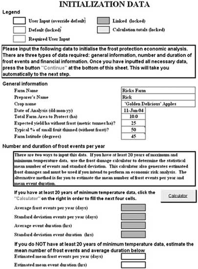
FIGURE 2.1b

Bottom section of Initialization worksheet

The user is required to supply eight elements of general information. Some of this information is solely for identification purposes (farm name, user, date prepared) but other elements (i.e. crop, protection area, expected yield without protection, typical percent of small fruit thinned, and farm latitude) are critical to subsequent analysis.

Number and duration of frost events per year are essential to determine whether the analysis proceeds as a cost-effectiveness or a risk analysis. There are two ways to input the number and duration of frost events per year. If at least 20 years of maximum and minimum temperature data are available, a "Calculator" button links the user directly to the frost damage calculator (see Chapter 1) to determine the statistical mean number of events and duration and their standard deviations. When sufficient weather data are not available, the user must estimate the mean number of frost events per year and mean event duration. Only one of the alternatives to input the average number of events per year and their average duration per night may be chosen. Since thirty years of data are available for this illustration, the damage calculator computed the mean and standard deviation of number of events (2.1 days and 1.9 days) and duration (5.5 hrs and 2.4 hrs), respectively.

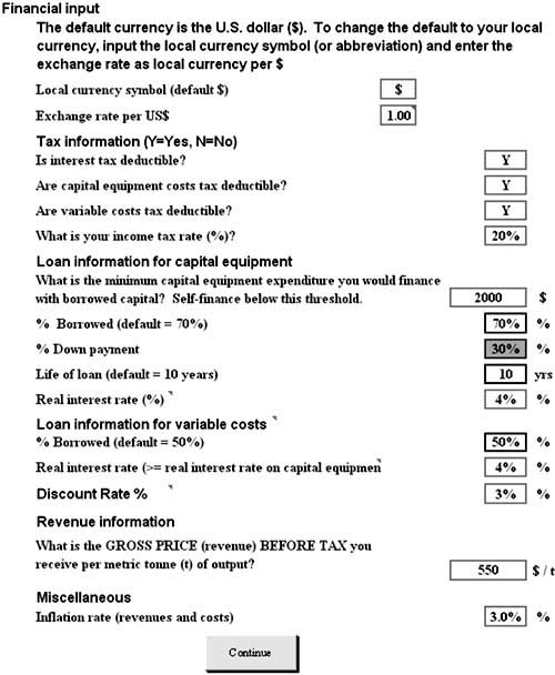
The final section of the initialization sheet involves financial data that are used to compute after-tax, annualized present value net benefits. This section is compartmentalized into seven subsections. Some input data are required from all users (red-boxed cells); other input data are not required from all users (black-boxed cells). Since elements of the seven subsections have not been previously discussed and are vital to understanding the subsequent economic analysis, each subsection is discussed below.

The default currency used throughout this program is USA dollars ($). Universal application, however, requires the flexibility to change the default currency to a local currency and automatically update all $ denominated values to local currency denominations. The currency is changed in two steps. First, a local currency symbol or name must be stipulated and second the exchange rate (i.e. the ratio of local currency to US$ 1) must be specified. If the local currency is $, it must be stipulated as such and the exchange rate is 1.00 (i.e. $/$). Once a local currency is specified, new currency symbols and monetized values reflecting the exchange rate will be applied automatically throughout the analysis.

After-tax calculations, if applicable, are based on the user-specified inputs provided in this subsection. As noted above, most middle- to upper-income countries collect income taxes from farmers. Often, the various costs of production (e.g. capital costs, annual operating or variable costs, and interest costs) are tax-deductible expenses that reduce income tax liability. Since this practice is not universal, initialization requires the user to stipulate whether any of the three types of expenses are tax deductible. The user is also required to stipulate the appropriate marginal tax rate as a percentage, 0 percent if no income tax applies.^[5] All expenses are tax deductible at a 20 percent rate in this example.

The next two financial subsections (loan information for capital equipment and loan information for variable costs) are essential to calculate the after-tax, annualized PV stream of expenses. Capital equipment may or may not be debt financed, depending upon the cost, and the cost threshold that defines when firms will debt finance equipment purchases differs across firms. Accordingly, the user is asked to specify various loan parameters. First, the user must specify the minimum capital equipment expenditure that would be financed with borrowed capital. Amounts below that threshold are assumed to be cash purchases. All amounts above that threshold are funded with a blend of borrowed funds and cash-down payment. An illustrative threshold of $ 2 000 is specified, but may be changed by the user. If the equipment is debt financed, the user must specify the percent of equipment expenditure borrowed (default is 70 percent); the down-payment percentage is calculated as (1 minus the fraction borrowed). Life of the loan also must be specified (default is 10 years). Finally, the interest rate must be specified as the "real interest rate" (i.e. market rate minus inflation rate). Use of the real interest rate simplifies subsequent financial calculations. The real interest rate on borrowed capital for equipment purchases is 4 percent in this example.

All variable costs may be financed with an operating loan or a line of credit against current-year production. It is assumed that the average draw on the line of credit is 50 percent, though the user may change this default. All variable expenses, including interest charges, are repaid in a single year. The real interest rate on the line of credit, 4 percent in this example, must be user specified and ordinarily is greater than or equal to the real interest rate on borrowed funds used to finance capital equipment.

The final piece of essential user-specified information is the before-tax, expected gross price (revenue) received per metric tonne (t) of output. This price is the weighted average price paid per tonne for fresh and processed apples. It is used in the calculation of frost protection benefits whenever a risk analysis is performed. In this example, it is assumed that the weighted average price of Golden Delicious apples is $ 550/t.

The user is also asked to specify the average inflation rate, though this information currently is not incorporated in the subsequent analysis. Upon completing the initialization data entry, the user should press the "Continue" button to move to the next sheet.

Technology Selection

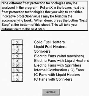
Nine frost protection technologies may be analysed with this program. However, not every technology is appropriate or of interest to every user. The user may select any or all of the frost protection methods to be analysed by placing an X in the box next to the protection method (Figure 2.2). Those methods left unchecked will not be analysed. It is important to understand that there is a cost to checking all technologies. While prototypical budgets are prepared for each technology, changes in budget elements are necessary to reflect local conditions and costs. For example, hourly wage rates must reflect local conditions. Equipment costs may also need to be tailored to local markets and to specific applications. Such changes are essential to prepare accurate cost-effectiveness or risk analysis of frost protection. The program is developed to provide a flexible and simple mechanical process to customize budgets. Nevertheless, acquiring location-specific cost data can be time consuming. All technologies are checked in the example.

Once the technologies are selected, the "Continue" button at the bottom of the TechSelect sheet should be pressed. The user will be taken to the budgets for each of the selected frost protection method, one at a time.

Budgets

The structure of budgets for each protection method is identical. Each budget begins with a restatement of data copied and locked from the first section of the Initialization sheet, followed by some method-specific initialization data that define the frost protection technology. For example, electric fan wind machines may be purchased in a variety of sizes and power units. If the default specification is considered inappropriate, the user may revise the fan-specific data to reflect the design being evaluated (e.g. the required number of size-specific fans for protecting the farm and the estimated °C of protection. Guidance concerning the degrees of protection offered by each method may be found in Chapter 7 (Volume I).

FIGURE 2.2

TechSelect worksheet

The body of each budget involves three additional sections: acquisition costs of equipment, annual variable costs and a total annual cost summary. Equipment acquisition costs and the annual variable operating costs must be adjusted to reflect that particular technology specification and unique application. The row labels in columns B and C define the various component cost elements; the associated unit costs, number of units per farm and total costs per farm are given in columns D to I. The Total Annual Cost Summary section has a slightly different format. Row labels are shown in columns B to F, and summary cost data are calculated in column I.

The budget process is illustrated in Figures 2.3.a and 2.3.b for a single frost protection technology: electric-powered fan wind machines. The user is encouraged to pay attention to all comments embedded in cells throughout the budgets. It should be remembered the numerical example is illustrative, reflecting a hypothetical 10-ha orchard application. Actual costs may vary widely from this illustration. Budget sheets for the other eight frost protection methods are provided in the Appendix.

FIGURE 2.3a

Top section of the budget sheet for electric-powered wind machines

FIGURE 2.3b

Bottom section of the budget sheet for electric-powered wind machines

Acquisition cost of equipment

This section of the budget (Figure 2.3.a) contains the total cost of purchasing equipment, itemized by row category. Freeze protection with electric fans requires a variety of investments. Each fan unit is comprised of a tower, fan, motor and control unit. Two 75 kW fan units are needed for the 10-ha apple orchard. Monitoring equipment includes a single freeze alarm for the entire farm, regardless of size, and one minimum thermometer per 5 ha. Particular applications may require "other equipment", which must be user defined. The first data column (D) contains default costs per unit, specified as $/unit. This column is hidden and write protected so that the user always has a reference point when tailoring the budgets. The second column (E) converts the hidden default cost per unit to local currency. Column (F) is to be used whenever the user wishes to override the default cost per unit (local currency). The default number of units required to protect the entire farm and the optional override are given in columns (G) and (H). The last column, (I), summarizes the row-specific category costs. Each cell in this column is locked (blue bordered) because each has an important formula that calculates the various subtotals. The bright blue shaded cell in column (I) is an aggregated category total, and is also a locked formula. The prototype presented here involves a $ 29 202 investment. The final element of this cost category is the expected equipment life (15 years). Although not a cost per se, the estimated equipment life must be specified for subsequent use in calculating after-tax, annualized PV costs in the summary section. The reader is cautioned that equipment life must match or exceed the loan period specified in Initialization.

Annual Variable Costs

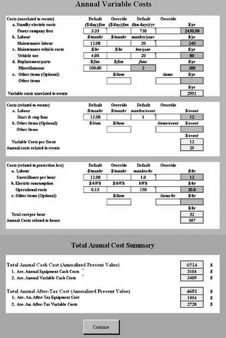
This section of the analysis (Figure 2.3.b) addresses the direct operating costs of frost protection. It is compartmentalized into three subsections of variable costs:

• costs unrelated to events (i.e. set-up costs);

• costs related to the number of events; and

• costs related to protection hours (i.e. event duration).

Electric fans incur at least four different variable costs unrelated to the number of frost events. Standby electricity costs are estimated to be $ 2 431/yr. Routine, off-season maintenance labour costs are $ 240/yr and the corresponding vehicle charge is $ 80/yr. Replacement parts average $ 200/yr. A fifth category, "other items", is an optional category provided in case the user wishes to specify additional set-up annual costs that are incurred in a particular application. Annual variable costs unrelated to events are estimated to total $ 2 951.

Electric-powered fans are capital intensive and involve little in the way of variable costs related to the number of frost events. It is estimated that only one hour of labour ($ 12) is required to start and stop the fans every time there is an event. A premium is included for night-time work. The user may specify an optional "other items" category. Annual variable costs related to the number of frost events total only $ 25, based on the estimated number of events (2.1 days) provided in the Initialization section.

As before, variable costs related to protection hours are first calculated on a per-unit basis (per hour) and then for the entire year ($/hr × hrs/event × events/yr). Variable costs that depend on event duration are surveillance labour ($ 12/hr) and electricity consumption ($ 20/hr). The default hourly labour charge assumes that a premium is paid for night-time work. Electricity charges are fan-size dependent and will vary widely across locations. The user may specify an optional "other items" category, as needed. Annual total variable costs related to protection hours are estimated at $ 367. This amount is the product of $ 32/hr × 5.5 hrs/event × 2.1 events/yr; the latter two elements come from Initialization.

Total Annual Cost Summary

The final section of the budget sheet (Figure 2.3.b) summarizes the total annual frost protection costs for the 10-ha apple orchard. Total annual cash costs are presented, followed by the total after-tax costs, both as annualized present values. The annualized cash costs lend insight into cash flow, whereas the after-tax costs measure the effective true cost of frost protection.

Total annual cash cost of frost protection with electric fans on this hypothetical 10 ha farm is $ 6 514, annualized PV dollars. This total cash cost is the sum of the average annual equipment cash cost and the average annual variable cash cost.

Average annual equipment cash cost depends upon whether the equipment acquisition costs were debt-financed or self-financed. If total capital acquisition cost exceeds the self-financing threshold specified in Initialization, then the annualized costs equal the sum of the down payment divided by the equipment life, plus the level principal and interest (P&I) payment on borrowed capital. Level annual payments imply the annual P&I payment is the annualized (i.e. financial average) value. If the equipment purchase is self-financed, then the average annual equipment cost equals the straight-line depreciation expense (i.e. total acquisition cost divided by the expected life). In this example, the cost of purchasing the electric fans exceeds the Initialization default threshold of $ 2 000, so the annualized equipment cash cost equals $ 3 104.

Average annual variable cash cost equals the level principal and interest (P&I) payment on the one-year, recurring line of credit. Recall the assumption that variable expenses are financed for a fixed, user-specified, percentage of a year (i.e. the average draw is a user-specified fraction of a year). The Initialization average draw default of 50 percent is used in this illustration. Average annual variable costs equal $ 3 409 (i.e. $ 3 343 in principal plus $ 66 in interest).

Total annual after-tax cost of frost protection with electric fans on this 10-ha orchard is $ 4 681 annualized PV. That is, the actual cost of this protection method is $ 1 833 less than the annualized cash cost because capital costs, variable costs and interest costs are all assumed to be tax deductible at a 20 percent tax rate (see Initialization data). More generally, the ratio of Total Average Annual After-Tax Cost to Total Average Annual Cash Cost decreases when capital costs are a smaller share of total costs. This general relationship is due to losing the after-tax benefit of capital purchases.

Like the calculation of cash costs, total after-tax cost is the sum of average annual after-tax equipment cost and average annual after-tax variable costs. The calculations for both of these component costs are dependent upon whether the user answered, "Yes" or "No" to the tax-deductible status of interest, equipment and variable costs. The average annual after-tax cost of equipment is further dependent on whether the equipment was debt financed.

Average annual after-tax equipment cost of electric fans in this illustration is estimated to be $ 1 954. This cost is calculated based on the fact that total equipment costs exceeded the self-financing ($ 2 000) threshold stipulated in Initialization and both capital and interest costs were stipulated as tax deductible. The conditional after-tax cost calculation used in this illustration involved the first of four alternative calculations.^[6]

1. If both capital cost and interest are tax deductible, the average annual after-tax cost is:

(1-TR) × (annualized PV interest + annual depreciation)

where TR is the tax rate; annualized PV interest equals the net present value of the stream of interest charges divided by the PV annuity factor; and annual depreciation is calculated as straight-line depreciation. The three remaining alternative conditional calculations are detailed here for completeness. Each assumes the frost protection technology is debt financed.

2. If capital cost is not deductible but interest is deductible, the average annual after-tax cost is:

(1-TR) × annualized PV interest + annual depreciation.

3. If capital cost is deductible but interest is not tax deductible, the average annual after-tax cost is:

(1-TR) × annual depreciation + annualized PV interest.

4. If neither capital nor interest costs are deductible, the average annual after-tax cost equals the average annual equipment cash cost. Note that if the self-financing threshold were not exceeded in any of the four calculations above, average annual equipment cost simply equals the straight-line depreciation expense.

Average annual after-tax variable costs for electric-powered fans are estimated to be $ 2 728. This cost is calculated in a conditional manner similar to the after tax equipment cost, though self-financing is not an issue. The conditional after-tax cost calculation used in this illustration involved the first of four alternative calculations.

1. If both variable cost and interest are deductible: (1-TR) × variable cost payment.

2. If variable costs are not deductible but interest is deductible: (1-TR) × annualized PV interest + total variable costs.

3. If variable costs are deductible but interest is not: (1-TR) × total variable costs + annualized PV interest.

4. If neither variable costs nor interest are deductible: average annual variable cost.

Upon completing each budget, the user must press the continue button to be taken to the next budget among those stipulated in the "TechSelect" sheet. Once the last budget is completed and the continue button is pressed, the user is taken to the first of two output reports: Cost-Effectiveness.

Cost-Effectiveness

At least 20 years of minimum and maximum temperature data are necessary to analyse the risk of frost damage. The user has to initialize the program with an estimate of the expected or typical number of frost events and duration. Then the economic decision defaults to the most cost-effective (i.e. lowest cost) method of achieving a given level of protection. Cost-effectiveness assumes that the number of frost events, their duration and extent of damage are known with certainty, presumably at a mean or expected level. This illustration is based on the mean number of events and duration generated by the damage calculator during the initialization step.

There are two output tables related to cost-effectiveness. The first (Table 2.1) is the first table in the CostEffectReport worksheet. This table ranks each of the nine frost protection methods in ascending order of the Annualized Present Value After-Tax Cost of Frost Protection by °C, regardless of the amount of protection. The last column indicates the annual after-tax cost per degree of protection, which highlights the fact that a lower cost method may, in fact, be an expensive way to achieve higher levels of frost protection. Stated differently, not all methods yield the same amount of protection; the lowest annualized cost of protection is not necessarily the best way to discriminate among alternative technologies.

Table 2.2, which corresponds to the second table in the CostEffectReport worksheet, lists the cost-effective methods of achieving minimum protection, ranked by annualized after-tax costs. This table presents a more comprehensive way to evaluate the cost-effectiveness of the nine different frost protection methods. The annualized after-tax costs for all methods that provide a minimum amount of protection are ranked in ascending order. For example, all nine methods offer at least 1 °C or 2 °C of protection. However, only seven methods offer at least 3 °C of protection, four protect against a 4 °C frost, and only three offer 5 °C or 6 °C of protection.

TABLE 2.1

Annualized present value (PV) after-tax cost of frost protection by °C

KEY: ICFan = internal-combustion0engine-powered fan. ElecFan = electic-motor-powered fan. LiqFuelHeaters = liquid-fuel heaters. SolidFuelHeaters = solid-fuel heaters.

TABLE 2.2

Cost-effective methods of achieving minimum protection, ranked by annualized after-tax costs

KEY: ICFan = internal-combustion-engine-powered fan. ElecFan = electic-motor-powered fan. LiqFuelHeaters = liquid-fuel heaters. SolidFuelHeaters = solid-fuel heaters.

Internal-combustion-engine-powered fans (ICFans) are shown to be most cost-effective but provide only 2 °C of protection. It has an expected annualized after-tax cost of $ 3 788. Electric-motor-powered fans (also offering only 2 °C of protection) are a close second at $ 4 681, followed closely by sprinklers (6 °C of protection) at $ 4 787. The proximity of sprinklers to the least-cost ICFan draws attention to an important consideration when using this cost-effectiveness table. Although the stochastic nature of frost protection is absent from cost-effectiveness, limited but crucial insight into risk management is possible. For less than $ 1 000/yr, sprinklers offer three times the protection of ICFans. Unless the user is very confident that frost events rarely exceed 2 °C, the appropriate technology based on a combination of costs and protection may be sprinklers, not the least-cost ICFan. The user should review all aspects of this second table to make the best possible economic decision, given the limited information.

If frost event and duration data were input in Initialization using the damage calculator, the user needs to depress the "Go to Risk Report" button located next to the first table. Note that this option is available without reviewing the cost-effectiveness results. The following discussion of risk begins with a conceptual overview of risk management because this is the heart of the decision to adopt frost protection. The discussion is followed by details illustrating the risk-minimizing choice among the nine alternatives considered in this analysis.

Risk

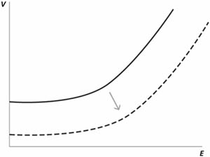
Decision-making under uncertainty has a long tradition in agricultural economics. At the centre of the risk literature is the problem of choosing among alternative risky actions or portfolios, whether choosing different crop rotations or hedging strategies that maximize expected earnings, while minimizing acceptable levels of risk. Assuming there is a probability distribution of revenues for all actions and this distribution can be defined adequately in terms of its first and second moments [i.e. mean or expected income (E) and associated variance (V)], then the choice among alternative actions may be conceptualized as a trade-off between net income expectations (commonly plotted on the horizontal axis) and net income variance (commonly plotted on the vertical axis). Greater risks imply greater income variability, which require greater expected payoffs to justify the risk. The set of so-called risk-efficient decisions lies on the mean-variance (E-V) frontier that is defined by the minimum variance (or standard deviation) for each level of expected income. As illustrated in Figure 2.4, the E-V frontier increases at an increasing rate (i.e. has positive first and second derivatives in the positive quadrant). Protection techniques with points above this boundary are dominated by methods on the risk-efficient frontier. Methods above the E-V frontier represent more risk (i.e. variance) for a given level of expected income or less income for the same level of risk.

FIGURE 2.4

Hypothetical E-V frontier without frost protection (—) and with frost protection (- - )

The optimal decision along this frontier differs from firm to firm, in accordance with firm-specific risk preferences that are functions of expected income and variance. Economists have dedicated considerable energy to the problem of soliciting and specifying risk preferences for individuals, with limited success. Inability to specify the risk preference function for every possible farmer simply means the framework precludes an optimal choice. Nevertheless, the E-V framework simplifies the choices confronting the decision-maker to those efficient ones on the frontier; all others are inferior to the profit-maximizing firm.

Frost protection extends the E-V framework in a straightforward way. Protection raises temperature, reduces damage and thereby increases expected yields and reduces yield variation. All else being constant, these physical benefits translate into increased expected income and reduced income variation (i.e. the benefits of frost protection). Providing the enhanced expected yield generates economic benefits that exceed the annual protection costs, the E-V-frontier with protection would lie below one without protection. Thus, adoption of frost protection offers the possibility of shifting the risk-efficient E-V frontier downward and to the right, providing that the net benefits (i.e. benefits minus costs) are positive. Deciding whether to adopt a method requires one to contrast the stochastic net benefits from the farming enterprise without protection against the stochastic net benefits with protection.

Two manifestations of risk must be accounted for when measuring net benefits of frost protection. There is yield risk attributable to the stochastic nature of weather (temperature, t) during different plant growth stages. This is sufficient to make revenues (i.e. gross benefits) from protection stochastic. There is also risk associated with the costs of frost protection, which includes both the annualized acquisition costs and the annual operating costs. The annual operating costs are related to the number and duration of frost events, both of which are stochastic and, in turn, functions of t. Recall that the variable cost of protection consists of three parts: variable costs unrelated to events; variable costs related to the number of events; and variable costs related to event duration. Thus, both benefits and costs are stochastic functions of the random variable, temperature.

Expected yield loss is a function of temperature, where the probability of a particular temperature is the weight assigned to the associated crop damage. One can think of two types of damage: total loss if the temperature, T, drops below T₁₀₀ or a continuously increasing loss function as temperature falls below T₀, until the entire crop is lost. Regardless of the type of damage function, one must first measure expected damages and associated variances with and without frost protection. The difference between maximum expected yield (Y) without protection, Y(T), and with protection, Y_z(T), varies by protection technology (z). Thus, [Y(T) - Y_z(T)] is the vector of stochastic yield damages and [Y_z(T) - Y(T)] is the vector of stochastic yield benefits. Maximum potential yield benefits correspond to the subset of z technologies offering the greatest elevation in temperature.

Stochastic yield benefits are translated into net economic benefits in two steps. First, net benefits (NB) without protection are defined as NB = P × Y(T), where P is the price of the crop grown net of all production costs except the cost of protection. Next, the vector of net benefits with protection (NB_z) requires a similar calculation, plus recognition that the operating costs of different frost protection methods depend on frost event frequency and duration, each of which is a function of T. Therefore, the method-specific cost of protection can be written as C_z(T). The vector of stochastic net benefits with protection is defined as NB_z = P [Y_z(T) - Y(T) - C_z(T)]. The frost protection method(s) yielding the greatest expected net benefit and lowest variance are risk efficient.

One need not examine the correlation or co-variation among the elements of risk (i.e. yield, events and duration) to measure composite risk. Instead, risk can be measured directly from the stream of net benefits. However, the nature of frost protection poses special challenges to measuring associated risk. The net benefit function is truncated from below and above, and probably is not a normal distribution.^[7] Closer examination of the frost protection process reveals why one cannot simply assume the net benefits are normally distributed and adequately characterized by first and second moments (i.e. the mean and standard deviation).

The decision to initiate protection on a given day must be made before frost is observed. That is, protection is started in anticipation of a frost event - at roughly +1 °C above the growth stage-specific critical temperature (T₀) - whether or not temperature continues to drop and protection is needed. This consideration means frost events are defined by, even though damage without protection might not occur. Alternatively, protection may be inadequate and either some crop damage occurs or the event is so severe (T £ T₁₀₀) that the entire crop is lost, despite protection efforts. Thus, one can think of net benefits from protection as falling into two categories: losses and gains, both of which have truncated distributions.

Losses occur whenever annual costs exceed benefits. Maximum potential economic loss for a given protection technology occurs in severe-weather years when protection is implemented but without benefit of any offsetting yield enhancement. Economic losses also occur in those years when the benefits of protection (the value of increased yield) are insufficient to offset the annualized acquisition cost plus operating costs. Losses also occur in those years when temperature never drops below critical levels, T > (T_o + 1 °C) capital acquisition costs are still incurred because the equipment must be paid for whether used or not and variable costs unrelated to the number of events (i.e. set-up costs) are also incurred. Gains in net benefits for any practice are similarly truncated from above at the value of maximum potential yield gain, less annual costs. Maximum net benefits for any given protection method occurs whenever yield without protection is zero (complete crop damage) but when maximum potential yield is realized because of protection.

The truncated nature of net benefit losses and gains, combined with the fact that it is doubtful whether the net benefit function arising from frost protection is normally distributed, renders a standard E-V table inadequate for farmers for evaluating the tradeoff between expected pay-off and the associated risk. Characterizing the likelihood of an incremental loss or a gain, in conjunction with the overall mean, provides a better decision-making tool. Accordingly, the approach taken here is to present the overall mean or expected net benefits and three additional parameters for losses and gains. Losses are characterized by the probability of loss, the expected (mean) loss, and the maximum loss. Gains are similarly characterized as the probability of gain, the mean gain and the maximum gain. These elements of a frost protection risk table enable the user to judge the merits of alternative risky investments in a manner that is analogous to an E-V table. The individual decision-maker has all essential information to evaluate the overall expected net benefit and the risk of loss or gain, given his or her risk preferences.

The trade-off between expected after-tax PV net benefits and risk associated with that payoff is summarized in Table 2.3, which corresponds to the first table in the RiskReport worksheet. Frost protection methods are ranked by the expected present value annual net benefits. The associated percentage probabilities of losses and gains, mean PV losses and gains, and maximum PV losses and gains are given. We begin the discussion of this table by first examining the risk elements associated with our example technology, electric fans, and then by examining the overall risk implications across all nine frost-protection methods.

The truncated nature of after-tax net benefits is illustrated by examining the detailed year-by-year after-tax net benefits without and with frost protection (not shown in Table 2.3). Maximum annual net benefits without protection is $ 110 000 under the assumptions specified in the Initialization data, the 30 years of weather data and the yield estimates derived from the damage calculator. Expected net benefits without protection equal $ 74 242, with a standard deviation of $ 48 257.

Table 2.3 shows that electric-powered fans, the illustrative example technology, are estimated to provide 2 °C of protection, generating an additional $ 26 797 of expected net benefits " the third-largest mean PV annual net benefit. The standard deviation of the additional net benefits, which is not shown in Table 2.3, is $ 45 640.

Closer examination of the year-by-year, after-tax net benefit from electric-powered fans reveals that a loss is more likely than a gain. A loss occurred in 17 of 30 years (i.e. 57 percent of the time), though the mean loss is only $ -4 528, while the maximum loss is $ -5 632. In seven of 30 years, protection was never implemented, resulting in an annual loss of $ -4 362; the annualized after-tax equipment costs ($ 1 954) plus the annualized after-tax P&I payment on variable costs unrelated to events ($ 2 408) still had to be paid. Protection was initiated in nine years, though no damage would occur even without protection.

TABLE 2.3

Frost protection methods ranked by expected PV annual net benefits and associated percentage probabilities of PV losses and gains, mean PV losses and gains and maximum PV losses and gains

KEY: ICFan = internal-combustion-engine-powered fan. ElecFan = electic-motor-powered fan. LiqFuelHeaters = liquid-fuel heaters. SolidFuelHeaters = solid-fuel heaters.

A resulting after-tax loss of up to $ -4 762 was incurred in these nine years. Finally, protection was implemented but did no good in one year, even though there were six frost events. Temperature dropped to the point of killing the crop, with or without protection, eliminating any possible yield benefits. In that one year, the after-tax annualized PV cost of protection was $ -5 632, the sum of all variable costs plus the annualized capital cost.

Turning to the gains side of protection, electric fans provided positive after-tax net benefits just 43 percent of the time. But the positive net benefits were large, averaging $ 67 760 and ranging up to a maximum $ 105 409 per year " just $ 4 591 less than maximum potential benefit. These results suggest that expected benefits from electric fan wind machines are associated with the risk of a relatively small loss but large potential gain. Electric fans are relatively risk free, despite the fact that 53 percent of the time protection is not needed and 3 percent of the time protection is not sufficiently effective to yield positive net economic benefits. Nevertheless, electric fan wind machines offer sufficiently large positive net benefits from frost protection the remaining 47 percent of the time to more than pay for themselves.

Before comparing risk across all nine-protection methods, it is instructive to detail the net-benefit calculations. First, all net benefits are after tax, unless capital and interest costs are defined in the Initialization worksheet as not deductible. Second, all benefits and costs are annualized PV. Annualized PV are the financial equivalent of average annual values expressed in current monetary units (i.e. removing the time value of money). Annualization allows a comparison among investments with unequal lives, as in the case of frost protection.

The after-tax annualized PV of net benefits is computed as the after-tax annualized PV revenues minus after-tax annualized PV equipment costs minus after-tax annualized PV variable costs. Annualized PV revenues are computed as the net price without frost protection, times yield per ha, times number of ha on the farm. Annualized PV equipment costs are computed as in the after-tax section of the budgets. Annualized PV variable costs comprise variable costs unrelated to events, variable costs related to the number of events and variable costs related to the number of events and the average event duration. These latter two variable cost categories differ from the budget calculations because the number and duration of events are year specific. Recall that the budgets were constructed on mean number of events and duration over the weather data series used in the damage calculator. Accordingly, year-specific variable costs comprise the sum of the three variable cash costs and the associated operating loan or line of credit interest. Use of real interest rates (i.e. net of inflation) makes the aggregate year-specific costs fully equivalent to annualized PV costs.

Each year of the weather data is treated as though it is a single, recurring observation of yield, events and duration, over the life of the particular frost protection method being analysed. Thus, the after-tax PV net benefits corresponding to a particular observation (year) are annualized PV net benefits over the life of the particular frost protection method. This analytical simplification avoids the problem of replacing different frost protection equipment at different times during the duration of weather data used in the damage calculator. Since each PV net benefit is annualized, average PV net benefits over all years of weather data are calculated as a simple mean. It follows that the additional $ 26 797 of expected net benefit generated by electric-powered fans is the simple average of 30 after-tax annualized PV net benefits. The expected after-tax PV net benefits for electric fans is similarly calculated, except each observation would reflect annualized PV net benefits for equipment that lasts 15 years, instead of, say, a 10-year life that might be expected from solid-fuel heaters.

Returning to Table 2.3, sprinklers (6 °C) offer the greatest overall mean PV net benefits, equal to $ 30 172, $ 3 375 more than electric fans (2 °C). The magnitude of potential losses and gains with sprinklers differs somewhat from electric fans, though the probabilities of gain or loss are within 3 percent of each other. Sprinklers have a slightly larger expected loss (i.e. $ -4 591 versus $ -4 528), though this protection method is exposed to a 16 percent smaller maximum annual loss than electric fans ($ -4 830 versus $ -5 632). The expected annual gains are $ 83 516, or roughly $ 1 400 more than with electric-powered fans. This greater gain is due to in part to the additional 4 °C of protection offered by sprinklers and in part due to the different cost structure. The additional 4 °C of protection was needed in only two years, but provided an additional 24 t/ha of apples. Maximum possible annual gain is similar between the technologies. Sprinklers offer a higher expected net benefit similar risk relative to electric fans, yielding comparable expected losses in years of loss and somewhat higher expected gains in years of gains.

Perhaps a more interesting comparison is between solid-fuel heaters (4 °C), the least attractive protection method, and sprinklers (6 °C). Even though solid-fuel heaters offer only 2 °C less protection, they provide less than one-tenth the expected annual net benefits ($ 2 319). Solid-fuel heaters are also more risky in the loss direction, but comparable in the gain direction. Solid-fuel heaters face a higher probability of loss (70.0 percent versus 56.7 percent) and incur a mean annual loss of $ -17 309 in contrast with $ -4 591. Turning to gains, solid-fuel heaters have a 17 percent lower probability of gain (30.0 percent versus 46.7 percent) and the expected gain is roughly half that of sprinklers (e.g. $ 48 118 versus $ 69 901). Maximum annual gain is also less.

Review of the remaining six frost-protection methods shows variations of the foregoing discussion of expected pay-off versus risk of loss or gain. Particular attention should be given to risk of loss because it can have serious detrimental impact on the financial well-being of a farmer in a single year or the ability to generate sufficient cash flow to pay off debt associated with frost protection. This observation is especially true when losses are more frequent than gains.

Table 2.4 depicts the second table in the RiskReport worksheet. It shows the relative risk associated with methods capable of providing 1°, 2°, °, 6 °C of protection. Frost protection methods yielding minimum protection are ranked in descending order by expected PV annual net benefits and the associated risk of annual loss or gain captured by the probability (the mean and the maximum loss or gain). Tables 2.3 and 2.4 reinforce an important feature of decision-making under risk. While it is both tempting and common to think in terms of achieving a given amount of protection, such an approach to the adoption decision is generally flawed. Even though the hypothetical farmer operates in an area where 2 °C of protection is inadequate to avoid all damage, a 2 °C technology (ICFans) may be the preferred investment.

Based strictly on expected net PV benefits, sprinklers dominate all other frost-protection methods. Sprinklers yield $ 2 460 greater expected net PV benefits than the next closest technology, ICFans. However, considering the exposure to risk makes the decision more ambiguous. Notice that sprinklers have a 25 percent higher expected loss and a slightly higher maximum loss. These two factors augur in favour of ICFans. Sprinklers do have a slightly higher mean PV gain, but ICFans have a larger potential maximum gain. The probability of losses (gains) is 3 percent lower (higher) for sprinklers.

The primary downside to sprinklers is the higher expected PV annual loss. This aspect of financial risk could be an important consideration to a farmer who is especially sensitive to a negative cash flow in any given year. The individual farmer must judge whether this adverse financial exposure is acceptable or too risky, given the upside tradeoff. If unacceptable, sprinklers might be less appealing than ICFans. Keep in mind that the numerical trade-off between expected PV annual net benefits and mean and maximum losses is unique to each application.

In summary, the risk analysis presented here differs from the cost-effectiveness analysis, in which methods were ranked according to least annualized after-tax cost. Recall that the ICFans wind machines (2 °C) were the least-cost protection method on the hypothetical farm. Sprinklers ranked third, with an annual cost 25 percent greater than that of ICFans. On a per-degree-of-protection basis, however, sprinklers ranked first, at $ 789/degree. This observation highlights the importance of tradeoffs among the economic benefits of protection, the level and structure of protection costs, and the risk of inadequate protection. If the user were obliged to make a decision based only on after-tax cost-effectiveness because sufficient weather data were not available to examine risk, considering the trade-off between cost and degrees of protection (a proxy for benefits) might lessen adoption errors. Such consideration would lead one to adopt sprinklers over ICFans, even though sprinklers are less cost effective. Nevertheless, sprinklers provide three times the protection (6 °C versus 2 °C). Notice that this slightly extended view of cost-effectiveness better approximates the choice of sprinklers that was guided by the risk analysis.

Other protection methods

Sample budget sheets for the other eight frost protection methods are given in the Appendix. All of the budget sheets represent protection of a 10 ha apple orchard with cv. Golden Delicious, which was used as an example in Chapter 2. A listing of the budget sheets by protection method is provided at the beginning of the Appendix.

TABLE 2.4

Frost protection methods yielding minimum protection ranked by expected PV annual net benefits (i.e. associated risk of annual loss or gain)

KEY: ICFan = internal-combustion-engine-powered fan. ElecFan = electic-motor-powered fan. LiqFuelHeaters = liquid-fuel heaters. SolidFuelHeaters = solid-fuel heaters.