1. First order subdivision: Geographical regions
2. Second order subdivision: LGP sub-zones
3. Third or subdivision: Agroglimatic sub-regions
4. Fourth order subdivision: Environmental units
5. Conclusion
The need for a regionalisation of the SAZ arises from its environmental heterogeneity (p. 2). A large number of variables is available, offering many alternative schemes. The interests of potential users have varying scale requirements, from continental divisions to sub-national administrative areas. To cope with this diversity, this Chapter develops a regionalisation of the SAZ of sub-Saharan Africa at four levels.
A first order subdivision is made between 'west and north' (W & N) and 'east and south' (E & S) regions on basic geographical properties. A second order subdivision of each region into four LGP sub-zones is based on data from the FAO. Population density, land use and potential population supporting capacities (with many intermediate variables) have been computed for these sub-zones on a country basis, and land inventory data on 16 soil constraints are available. Recognising that country-based LGP zones are not ideal for all purposes, a third order subdivision into sub-regions (16 in number) is based on three broad agroclimatic criteria: moisture and rainfall regimes and the monthly patterns of peak rainfall. At this level, some modifications are proposed to the SAZ as delimited by the FAO. Finally, the sub-regions are broken down into fourth order environmental units, 83 in number.
This subdivision embodies the contrast between the relative uniformity and continuity of the W & N region on the one hand, and the diversity and discontinuity of the E & S region on the other. At a gross level of generalisation, the W & N region (from Senegal to the Sudan) can be characterised in terms of the following properties:
(1) a lowland plains topography;(2) a uniform, unimodal rainfall regime;
(3) a transitional location between the Sahara Desert and the Subhumid Zone, reflected in a strong latitudinal bias in most ecological distributions;
(4) spatial and ecological continuity across its entire breadth;
(5) horizontal (south-north) aridity gradients and associated dispositions of tsetse;
(6) a history of cultural interaction, including the co-residence, in the same territories, of specialist pastoralists and farmers, with resource-sharing agreements;
(7) an absence of colonial land alienation, and the spatial continuity of its farming systems.
The SAZ of eastern Africa is very different, having:
(1) both highland and lowland areas;(2) both bimodal and unimodal rainfall regimes;
(3) a weak relationship between ecology and latitude, and abrupt ecological gradients, owing to highlands;
(4) a discontinuous spatial distribution;
(5) both vertical (altitudinal) and horizontal (multi-directional) aridity gradients, and complex associated patterns of tsetse challenge;
(6) a lack of notable historical uniting influences, with pastoralists and farmers often separated and competing for resources;
(7) extensive land alienation under colonial rule (in some countries), and discontinuous, diverse, sometimes isolated, or administratively confined farming systems.
The SAZ in southern Africa does not conform in all respects with the eastern African pattern. There is less highland, stronger latitudinal control, and more consistent ecological gradients. But it contains a comparatively small proportion of the African livestock (and human) populations. Since the E & S region is defined essentially in terms of its diversity, it makes practical sense for present purposes to include southern with eastern Africa, at this level of generalisation,
It is implicit in the foregoing that there are limits to the transferability of research and experience between the W & N and the E & S regions.
FAO land inventory data, and variables used for estimating population supporting capacities in the study carried out jointly by the FAO and IIASA (FAO, 1980; 1982), are available for LGP sub-zones broken down by thermal zone and by country. The sub-zones are:
|
M 1 |
150-179 growing days |
|
M 2 |
120-149 growing days |
|
D 1 |
90-119 growing days |
|
D 2 |
75-89 growing days. |
The thermal zones that occur in sub-Saharan Africa are:
|
MC 1 |
Warm tropics |
|
MC 2 |
Moderately cool tropics |
|
MC 3 |
Cool tropics |
|
MC 7 |
Warm sub-tropics (summer rainfall) |
|
MC 8 |
Moderately cool sub-tropics (summer rainfall) |
|
MC 9 |
Cool sub-tropics (summer rainfall). |
When overlaid on national territories, the variables listed above generate a three-dimensional matrix of more than a hundred cells. The data relevant to the present study are summarised in Appendix 3. These have been selected from a list of 16 soil constraints and 29 population and productivity related variables.
Leaving aside the thermal zones, which have less relevance for livestock production systems, some of the data on the LGP sub-zones are aggregated at the regional level in Table 3.1. The FAO offers the only source of standardised physical land inventory, land use, and productivity data for all of sub-Saharan Africa, though the time-base for these data is 1975, and their reliability can be no better than that of the primary sources used.
According to FAO (1978: 98-9) the growing periods are classified as follows with regard to agroclimatic suitability for the major crops, pearl millet, sorghum and maize, at existing (low) input levels:
|
LGP (days) |
75-89 |
90-119 |
120-149 |
150-179 |
|
Pearl millet | ||||
|
Yield (t/ha) |
0.3-0.4 |
0.5-0.8 |
0.5-0.8 |
0.7-1.0 |
|
Suitability |
MS |
S |
S/VS |
VS |
|
Sorghum: | ||||
|
Yield (t/ha) |
|
0.3-0.5 |
0.5-0.7 |
0.9-1.3 |
|
Suitability |
NS |
MS |
S |
VS |
|
maize: | ||||
|
Yield (t/ha) |
|
0.4-0.5 |
0.7-1.0 |
1.2-1.8 |
|
Suitability* |
NS |
MS |
S |
VS |
* Suitability classes: NS - not suitable; MS - marginally suitable; S - suitable; VS - very suitable.
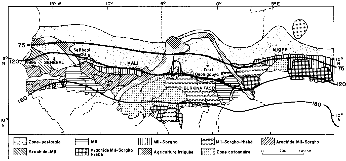
In the two drier sub-zones (75-119 days LGP), millet is the most suitable staple crop. However, the correspondence between these suitability ratings and actual practice may not be very close. For example, if the LGP isolines are superimposed on a map of major crop regions in the Francophone West African countries (Figure 4), it appears that other factors besides agroclimatic suitability (so defined) have influenced the pattern.
TABLE 3.1 The SAZ of sub-Saharan Africa by length of growing period (LGP) zone
|
|
W & N Region |
E & S Region |
All Regions |
Total |
|||||||||
|
M1 |
M2 |
D1 |
D2 |
M1 |
M2 |
D1 |
D2 |
M1 |
M2 |
D1 |
D2 |
|
|
|
Total area (000km2) |
|
|
|
|
|
|
|
|
1,822 |
1,207 |
1,311 |
856 |
5196 |
|
Population (1975, millions) |
|
|
|
|
|
|
|
|
31.2 |
26.7 |
17.1 |
11.2 |
86.2 |
|
Density (persons/km2) |
|
|
|
|
|
|
|
|
17.1 |
22.1 |
13 |
13.1 |
16.6 |
|
Agricultural land available (000 km2) 1 |
934.8 |
660.4 |
484.1 |
402.7 |
587.7 |
379.1 |
733 |
384.4 |
1,522.5 |
1,039.5 |
1,217.1 |
787.1 |
4566.2 |
|
Cropland (rainfed and irrigated: 000 km2) 2 |
787 |
457.5 |
129.1 |
90.2 |
469.9 |
298.9 |
170.6 |
130.4 |
1,256.9 |
756.4 |
299.7 |
220.6 |
2533.6 |
|
Rangeland (000 km2) |
30.6 |
115.5 |
287.9 |
262.1 |
45.3 |
119.8 |
424.8 |
234.1 |
75.9 |
235.3 |
712.7 |
496.2 |
1520.1 |
|
Percent cropland |
84 |
69.3 |
26.7 |
22.4 |
80 |
78.8 |
23.3 |
33.9 |
82.6 |
72.8 |
24.6 |
28 |
55.5 |
|
Percent rangeland |
3.3 |
17.5 |
59.5 |
65.1 |
7.7 |
31.6 |
58 |
61 |
5 |
22.6 |
58.6 |
63 |
33.3 |
Source: FAO (1982): 109, 115.1 The amount of agricultural land available allows for deducting estimated nonagricultural land from total land.
2 Cropland and rangeland do not add up to agricultural land available. We assume that the balance is unused.
See Appendix 2.
Functions linking LGP sub-zones with livestock-related variables have not been developed. Two variables of obvious importance are pasture production and availability of suitable crop residues. On the first, Le Houérou (1985) has proposed a link between annual rainfall and the production of dry matter above the ground, or rain use efficiency factor (RUE: kg DM mm-1ha-1yr-1). Studies in the Sahel yield averages ranging from 2.2 to 3.6, and in East Africa, from 3.2 to 6.0. He cautions, however, that differences in the length of the growing season between the unimodal rainfall regimes of the Sudano-Sahelian region and the bimodal regimes of East Africa cause fundamental differences in range type, composition and forage quality during the annual cycle. More work is therefore necessary before linkages between LGP and forage availability can be stated with any confidence.
Moisture regimes
Unimodal and bimodal regimes
Monthly patterns of peak rainfall
Functional definition of the SAZ
The sub-regions
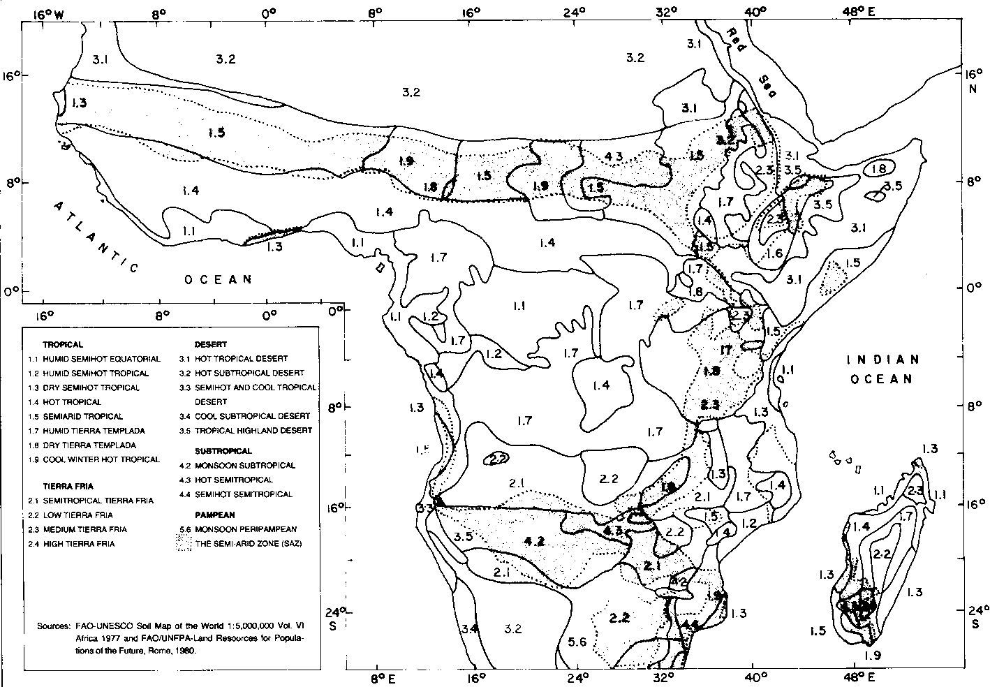
Sub-zones based on the use of LGP as a sole criterion do not take account of other agroclimatic variables. Thermal zones, or a general climatic classification, could be used to break the SAZ down into smaller units having more internal homogeneity. Figure 5, for example? shows the SAZ superimposed on a climatic classification employed for the Soil Map of Africa (UNESCO, 1977). No less than six tropical climates, three sub-tropical, two 'tierra fria' and a desert climate are represented. Or, the six thermal zones of the FAO land inventory could be used. But the relevance of general climatic classifications, or thermal zones, to livestock production is less evident than that of individual variables. Of these, the most important are moisture regime (LGP), modal type (unimodal versus bimodal regimes), and monthly patterns of peak rainfall.
The FAO (1990) has recommended that the 120-day LGP isoline should demarcate the moist from the dry semi-arid zones:
|
Dry semi-arid |
75-119 days growing period |
|
Moist semi-arid |
120-170 days growing period |
Figure 5. The SAZ in relation to major climates, after FAO (1980).
This two-fold division of the SAZ has greater practical utility than the fourfold division used in the preceding section since it reflects noticeable differences in livestock management in many areas. These differences are most apparent in the W & N region which is characterised by relative homogeneity from east to west and an ecological gradient from south to north. Therefore it is proposed to divide the W & N region into two sub-regions, Moist W & N and Dry W & N. In the E & S. the same distinction produces a complex spatial pattern having less usefulness for regional subdivision, though the importance of such distinctions for farming systems is clear at the micro-regional level (see, for example, Jaetzold and Schmidt, 1982).
This property has a significance for farming systems second only to that of the growing period. Following Leroux (1983), the SAZ can be subdivided on this basis. Unimodal regimes occur throughout the W & N region (with the exception of a small area of Mauritania, which it has been decided to ignore), and in NW Ethiopia, in the E & S region. Bimodal regimes occur throughout the E & S region from NE Ethiopia to Tanzania. From Tanzania (which is transitional) until the Tropic is reached, unimodal regimes occur. In the sub-tropical part of the E & S region, unimodal regimes occur in S. Mozambique, E. Swaziland, and Madagascar, but complicating factors extend the length of the rainy season in S E Botswana and W. Lesotho.
In the W & N region, under unimodal regimes and strong latitudinal influence, August is the peak month in normal years. In the E & S region, the latitudinal range of the SAZ (from 15°N to 30°S), and the influence of highland masses, create considerable variability in the monthly patterns of peak rainfall. These variations need to be taken into account in proposing sub-regions of homogeneous agroclimatic properties.
Before combining the above three variables into a scheme of agroclimatic sub-regions, it is appropriate to examine some anomalies in the definition of the SAZ which arise near the upper (180 days LGP) and lower (75 days LGP) limits. In several locations the reliability of these limits, as indicators of semi-arid ecological conditions for farming systems, may be questioned.
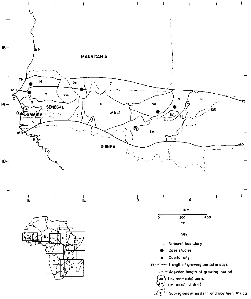
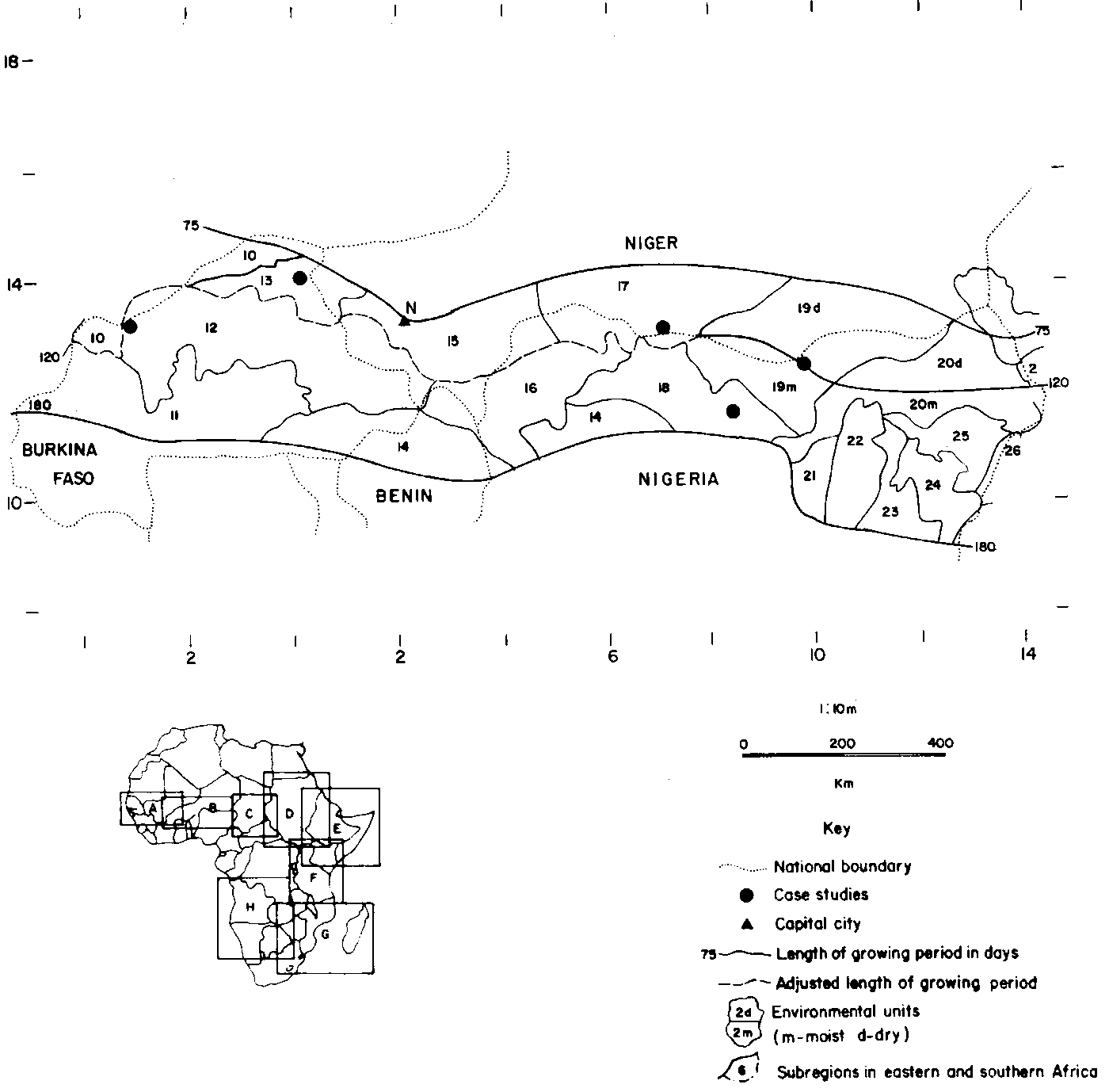
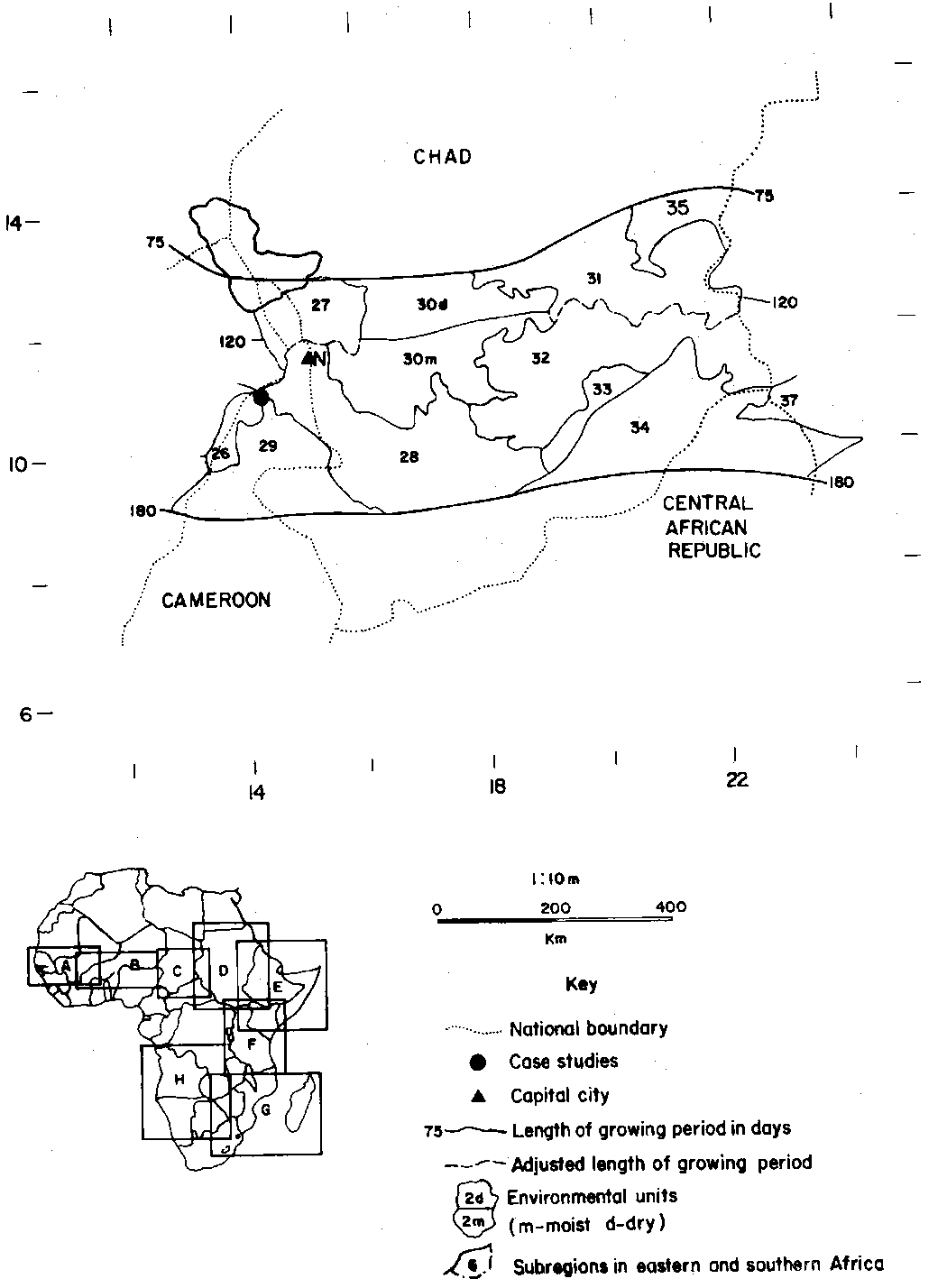
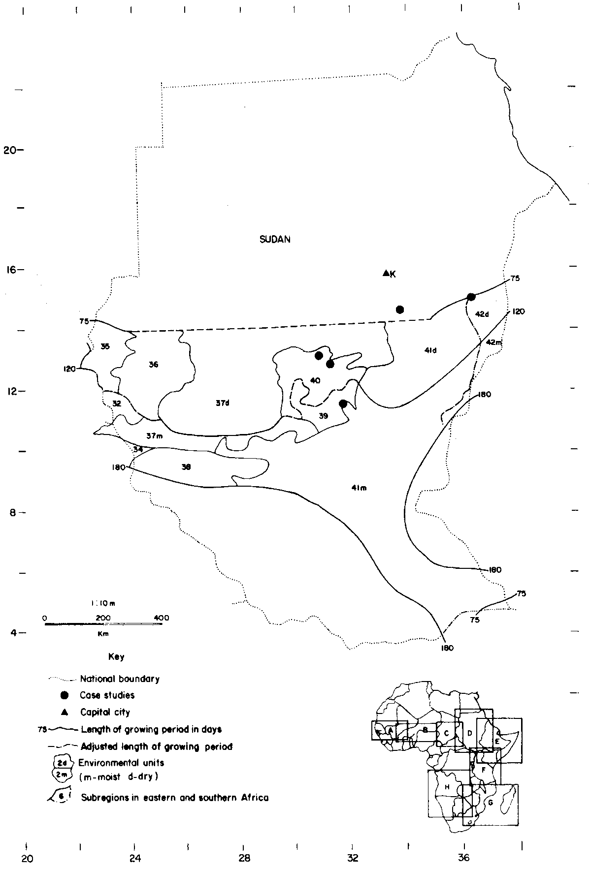
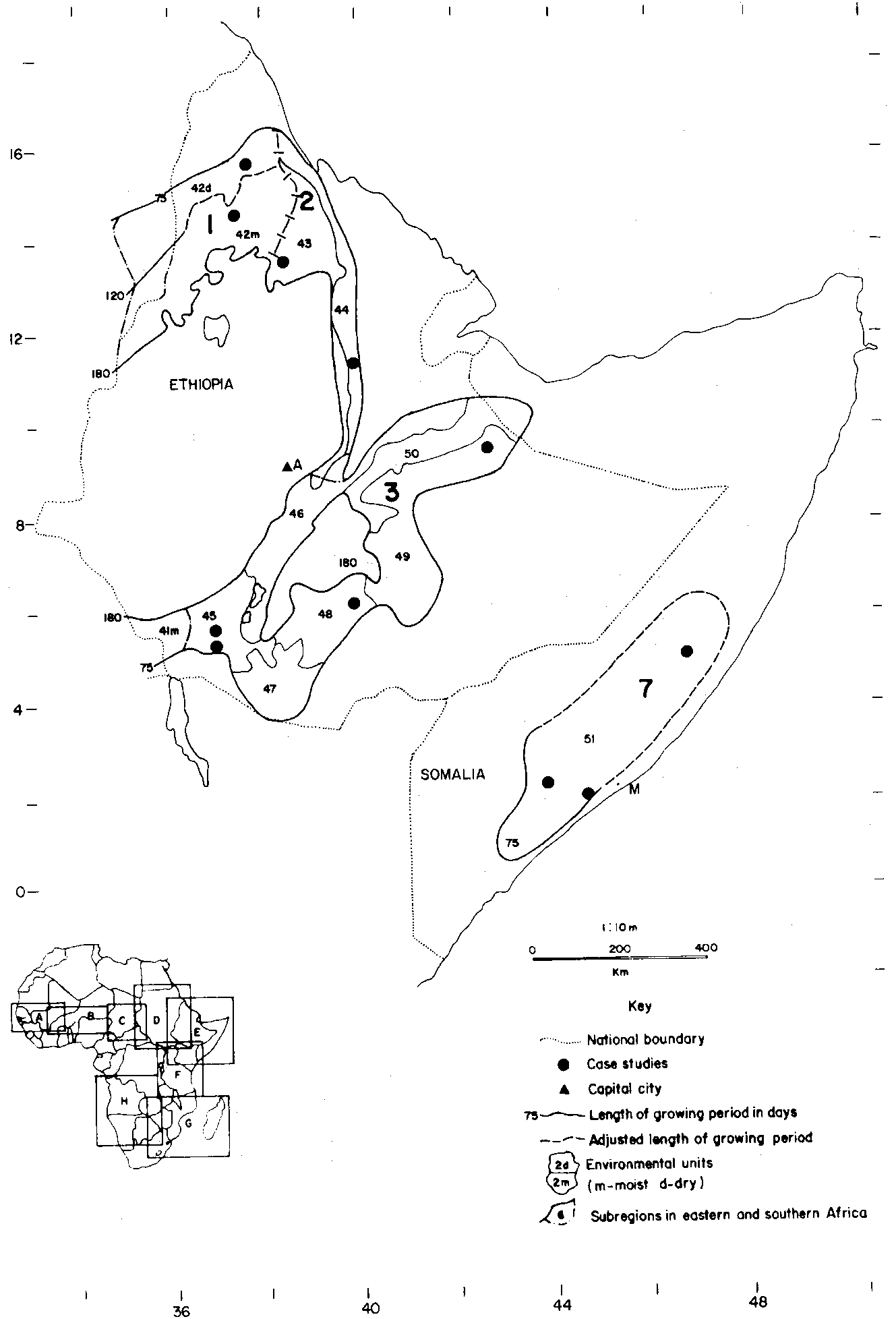
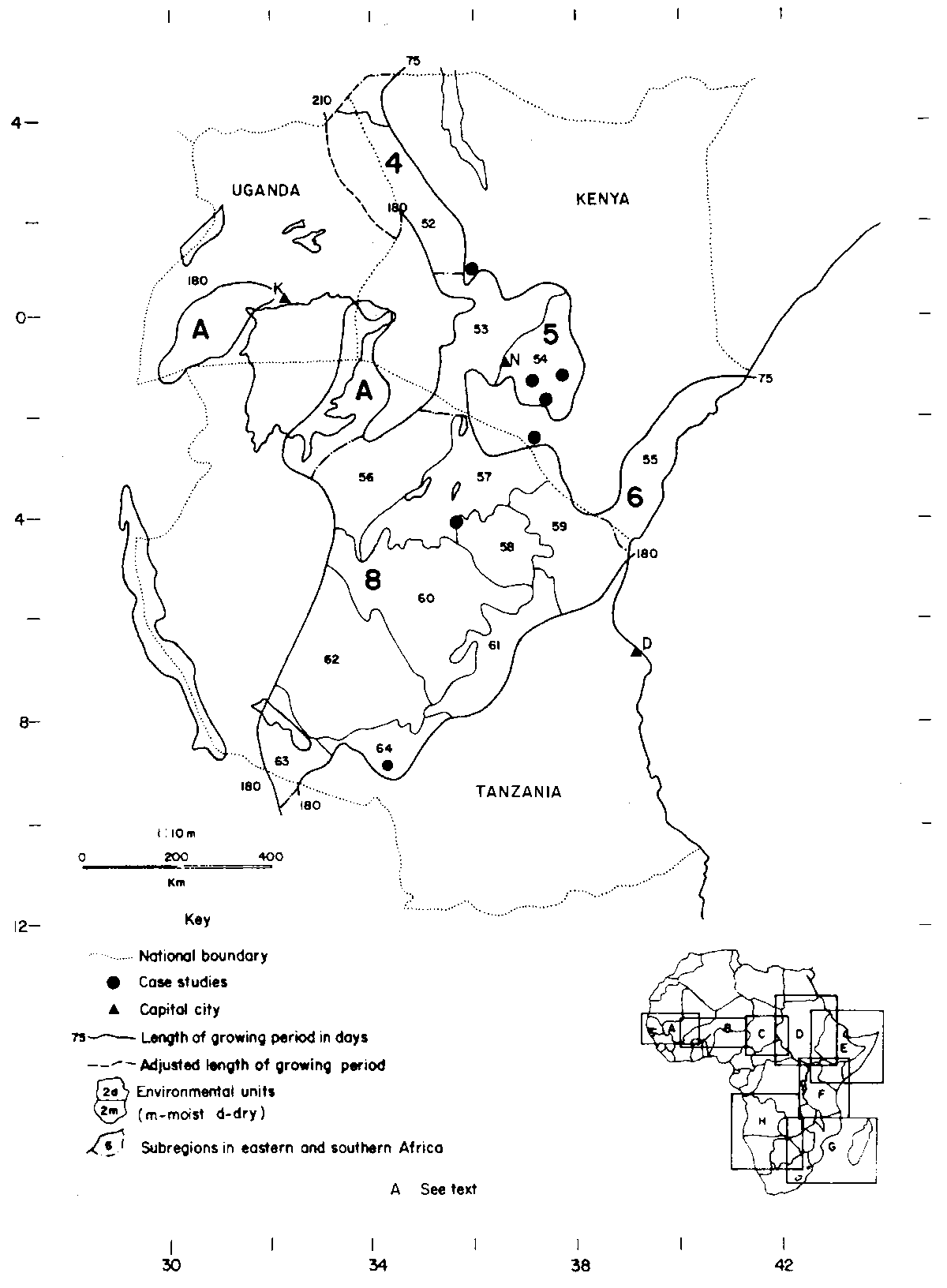
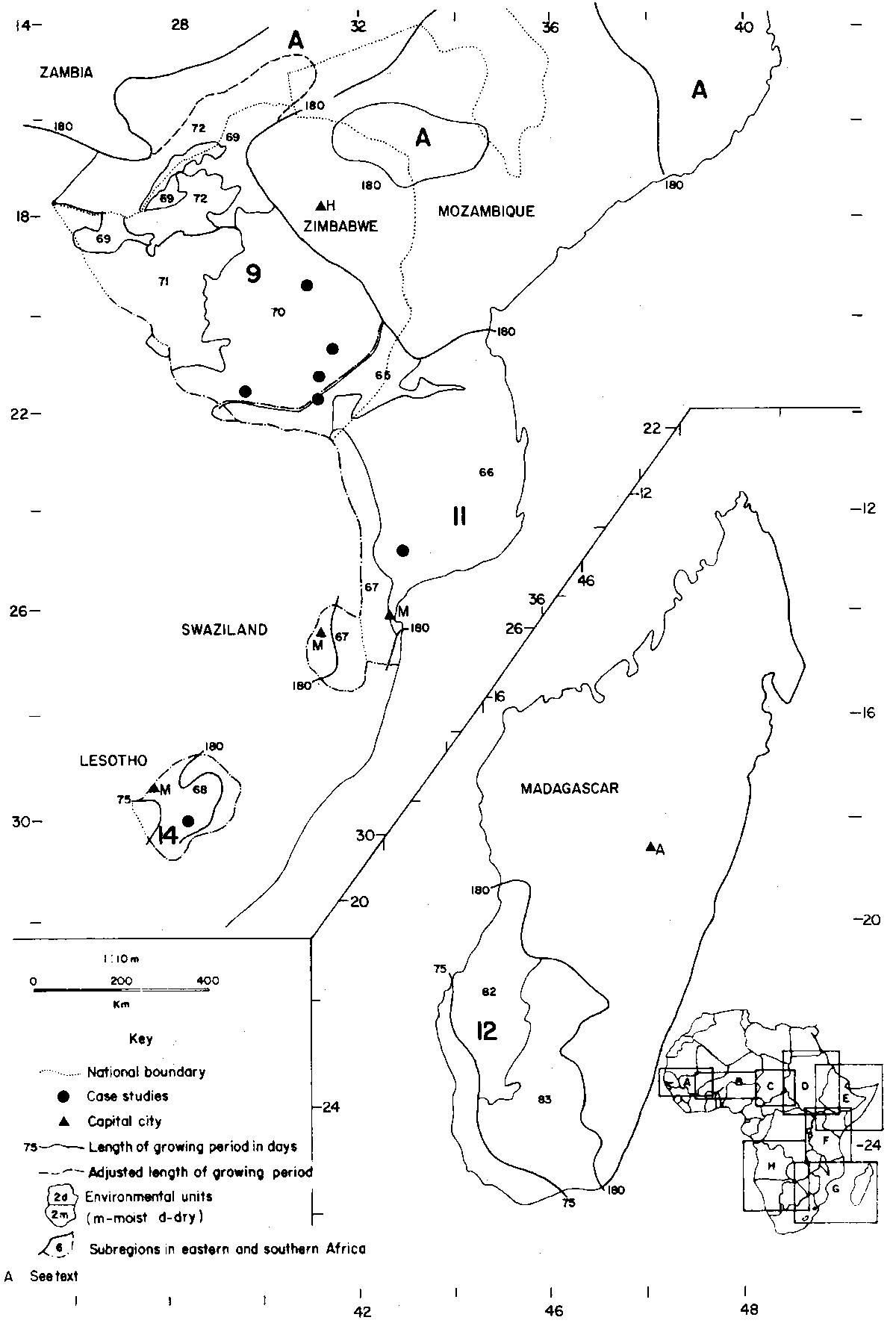
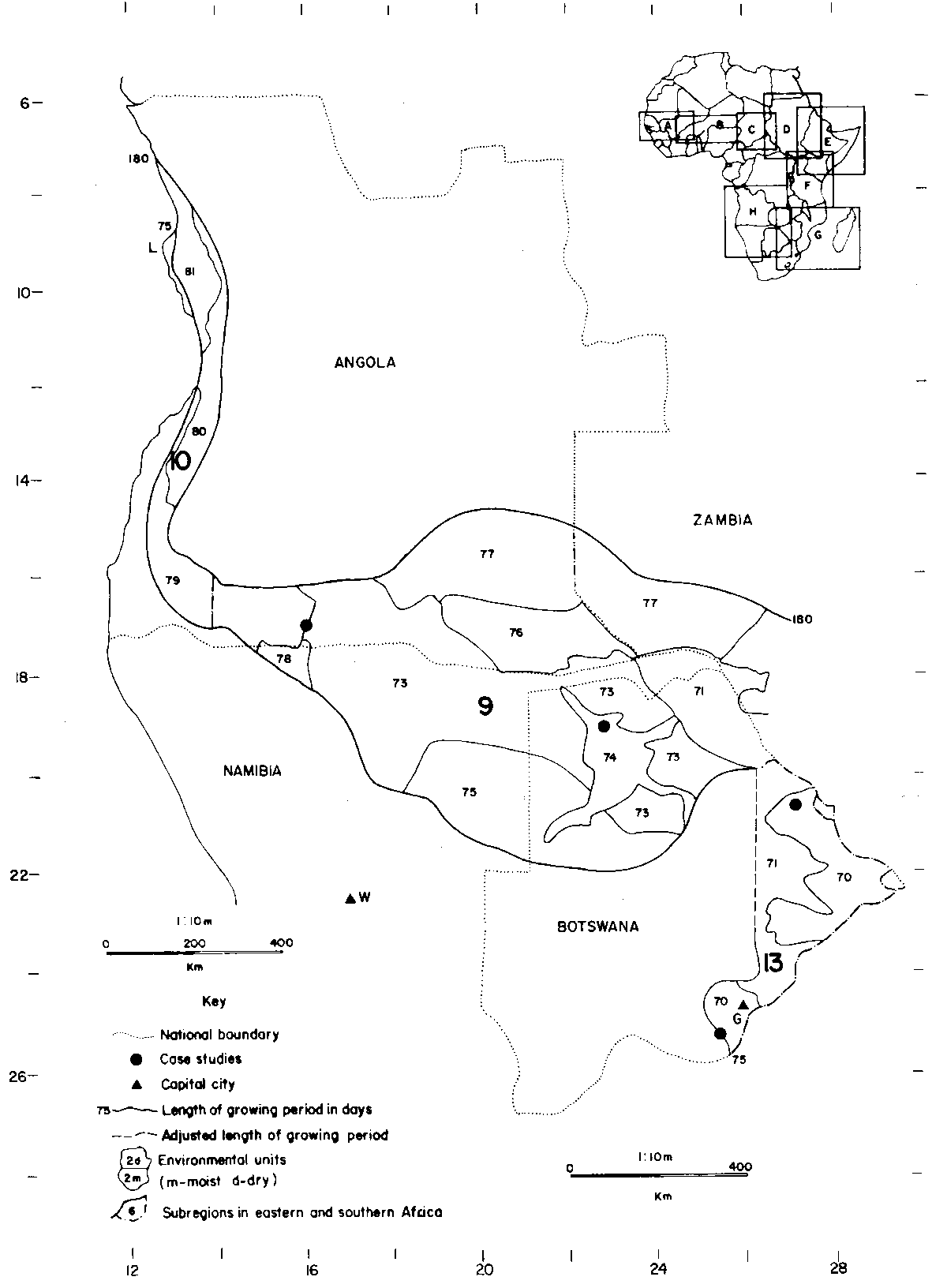
The following functional modifications to the SAZ are therefore proposed, for the reasons given (see Figure 1; and the boundaries shown in Figure 6 (A-H):
(1) W & N region, arid boundary; rainfed farming occurs extensively on the north side of the 75-day isoline in the Sudan, and sporadically elsewhere. On the Qoz Sands of Kordofan, rainfed cultivation extended beyond 14° until 1980 (Olsson, 1985). This line is proposed instead as a functional limit (Figure 6D).(2) E & S region, Kenya-Uganda borderlands: NE Uganda (Karamoja) received 650-850 mm of rainfall during the first half of the present century, characterised by extreme variability, supporting a vegetation of dry thorn scrub and a mixed pastoral-farming economy with cattle keeping both economically and culturally dominant. From Dyson-Hudson's (1966) account, it appears that the whole area (except possibly the mountains), up to the 210 day isoline, is best described as semi-arid. The boundary has been adjusted to include this area (sub-region 4, Figure 6F). On the Kenyan side of the border, almost all the territory with 75 or more growing days is rated as arid, with a very low stock carrying capacity, in Kenyan ecological classifications (Bekure et al., 1987). (Sub-region 4, Figure 6F).
(3) E & S region, S Somalia: rainfed agro-pastoralism extends well beyond the Bay region of southern Somalia to the central rangelands between 3° and 5°N (Holt, 1986). Rainfall, although low, is distributed through a long season. It is proposed to extend the functional boundary to include this area (Sub region 7, Figure 6E).
(4) E & S region, W Kenya and SW Uganda: notwithstanding anomalously short growing periods (less than 120 days according to FAO), ecology and farming systems in the environs of Lake Victoria are subhumid in character (Mwendwa, 1985); in the Kenya portion only a small strip of territory receives less than 800 mm of rainfall annually. Both these areas, with the Lake Victoria coast of Tanzania (shown as A on Figure 6F) are excluded from our functional definition of the SAZ.
(5) E & S region, Zambia: there are major differences between the LGP zones according to FAO and those estimated by an independent country study (Muchinda, 1985: see Appendix 6). These latter indicate shorter growing periods. Nevertheless, the ecology of most parts of Zambia is not semi-arid, and the farming systems (Schultz, 1976) have more in common with subhumid systems elsewhere. Altitude and latitude, through the temperature regime, must influence the effectiveness of Zambian rainfall, which appears to have a different relationship between annual total precipitation and length of growing period (more rainfall, shorter GPs) than is observed generally in the SAZ. For present purposes, Zambia is excluded from the SAZ, together with adjacent territory in Malawi (shown as A on Figure 6G).
(6) E & S region, Tanzania: certain areas in central Tanzania falling below the 75 day isoline are included in the SAZ on the grounds of their relatively small size and fragmented pattern (Sub-region 8, Figure 6F).
(7) E & S region, N & W Mozambique: the first of these zones (N Mozambique) carries a broad-leafed woodland, is heavily infested with tsetse, only moderately populated and appears to have few livestock (Timberlake and Jordao, 1985: 5). The second is a small, sparsely inhabited area almost devoid of livestock. Although no farming system characterisations have been found, it is believed that they are neither truly semi-arid nor significant to the livestock economy of Mozambique, and they are therefore excluded (Shown as A on Figure 6G).
(8) E & S region, E Botswana: the 75 day isoline understates the extent of rainfed farming in E Botswana significantly (while possibly overstating it in the north); excluded farming areas in Palapwe and Tutume should be included in the functional definition, which is extended westwards to 26°E (Sub-region 13, Figure 6H).
These revisions made, the sub-regional classification is tabulated below and shown in Figure 6 (A-H).
|
Rainfall regime 1 |
Subregion number 2 |
Subregion |
Rainfall peak months: |
|
|
W & N |
Single |
Double |
||
|
A |
- |
Dry semi-arid |
Aug |
|
|
A |
- |
Moist semi-arid |
Aug |
|
|
|
|
E & S |
|
|
|
A |
1 |
NW Ethiopia |
Aug |
|
|
B |
2 |
NE Ethiopia |
|
Mar-Apr: July-Aug |
|
|
3 |
S Ethiopia |
|
April: Oct |
|
|
4 |
N Kenya |
|
Apr-May: Jul |
|
|
5 |
E Kenya |
|
April: Nov |
|
|
6 |
Coastal Kenya |
|
Apr-May: Nov |
|
|
7 |
S. C Somalia |
|
Apr-May: Oct-Nov |
|
|
8 |
Tanzania 3 |
Jan |
Mar-Apr: Dec-Jan |
|
A |
9 |
Southern tropics(S Zimbabwe-N Botswana-NE Namibia-S Angola) |
Jan-Feb |
|
|
|
10 |
Coastal Angola |
Mar |
|
|
C |
11 |
Southern sub-tropics (S Mozambique, E Swaziland) |
Jan-Feb |
|
|
|
12 |
SW Madagascar |
Jan |
|
|
|
13 |
SE Botswana |
|
Oct-Apr 4 |
|
|
14 |
W Lesotho |
|
Dec-Mar 4 |
1 A: unimodal; B: bimodal; C: subtropical.2 Subregion numbers are shown in Figure 6 (A-H), where they are further sub-divided into environmental units (see below).
3 In Tanzania there is a complex transitional pattern of bimodal and unimodal regimes.
4 No clear peak in a long sometimes irregular. rainy season.
The foregoing regional subdivisions leave much environmental diversity unaccounted for, being confined to agroclimatic variables. Soil-related variables need now to be conjoined with other relevant variables in order to delimit smaller units having a greater degree of homogeneity with regard to the primary resources of farming systems.
In principle, a GIS-overlay computerised technique offers a method of unifying the variable distributions of different data sets. The nearest approaches to an operational GIS including environmental variables in sub-Saharan Africa are the FAO Land Inventory and UNEP's GEMS development. In the time available for the present study it has not been possible to explore the capability of the GEMS. The FAO Land Inventory has been used in Section 2 (above) to catalogue certain variables against LGP sub-zones. As mentioned above, the LGP sub-zones, when overlaid on thermal zones and countries, generate over 100 cells. If the soils map is superimposed on the map of LGP sub-zones, the number of cells is excessively large - 1,213 for Kenya alone (FAO, 1984: 2). Something much simpler is needed for present purposes.
The sources for this exercise are published maps. Those used were:
1. Soil map of Africa, 1: 5M (FAD/UNESCO, 1977)
2. Soil degradation risk, 1: 5M - Africa north of 2°N only (FAO/UNEP/UNESCO, 1980)
3. Grassland communities, 1: 10M (FAO, 1960)
4. Vegetation Map of Africa, 1: 5M (UNESCO/AETFAT/UNSO, 1981)
5. Desertification risk, 1: 25M (UNEP, 1977)
6. Tsetse distribution, 1: 5M (STRC, 1973)
7. Cattle density, 1: 10M (IBAR, 1988)
8. Population density, 1: 10M (USSR, 1968)
The objective is to search the patterns of the mapped variables for convergent spatial distributions that provide a basis for environmental units. Land inventories have been developed, and published, for a number of national and sub-national areas including or impinging on the SAZ of sub-Saharan Africa. The resources available for such studies (e.g. those conducted by the LRD/LRDC/ODNRI/NRI of the UK Overseas Development Administration, the IEMVT in France, and the FAO/UNDP) permitted the processing of large quantities of primary data - air photography, soil samples, etc. - and their incorporation into hierarchical procedures for taxonomy and aggregation of environmental units (cf. Bunting, 1987). These cannot be used for present purposes, because there is no way of bridging the gaps, or ensuring zonal compatibility.
The present attempt at a preliminary approximation of environmental units for the SAZ relies, therefore, on a manual assessment of output from the sources listed above. There are many anomalies in the data which could not be solved given the time available. Also, the benchmark dates of the sources vary from the 1960s to (perhaps) the 1980s. A hazard that is intrinsic to any attempt to evaluate environmental trends is that such benchmarks may not be made clear in the sources, and in any case such data compilations have to make use of primary studies differing in date and reliability. The least reliable data probably affects the population, livestock and land use estimates. Desertification risk classes also cannot carry much weight, since only the briefest description is given of the method used to derive them (UNEP, 1977). There are anomalies apparent on several of the maps.
The method used is as follows:
(1) The 75 and 180 day LGP isolines are superimposed on country sections of the Soils Map of Africa at 1: 5M.(2) Generalised soil units are derived in three classes:
1. one soil dominant >50% area (with or without associated soil >25% area)
2. two soils dominant, total >66% area
3 no soils dominant (complex pattern).
It should be noted that the map units shown on the Soils Map of Africa are associations of dominant, associated, and included soils, and that each of the 20 soil classes used is further subdivided into several soil units. In order to simplify, we used only the soil class (designated by a capital letter) and reduced the number of classes from 26 to 17 by omitting 9 classes considered to have minor importance in the SAZ. For example, Environmental Unit 35 in Sudan has associated soils described as follows:
I/R + J
i.e., a dominant soil class, lithosols (I) with regosols (R) - >50% area occurs with an associated soil class, fluvisols (J) - >25% area.
(3) If the 120-day isoline bisects the unit thus recognised, it is subdivided into two, identified as d (dry) or m (moist). If the isoline divides the unit very unequally, the lesser part is included under the dominant moisture regime.(4) Where data are available, a degradation risk value is assigned to the unit.
(5) The dominant grassland community and descriptive category (e.g. savanna) are recorded, followed by the vegetation class number and a summary description of the woody vegetation.
(6) The dominant desertification risk category is recorded.
(7) An estimate of cattle density in each unit is obtained by choosing a representative 1 cm2 (10,000 km2 at 1: 10M) and counting the dot symbols.
(8) The units are overlain on the population density map and the dominant range estimated, omitting urban and pert-urban agglomerations.
(9) The presence of tsetse and species is recorded.
(10) The environmental unit boundaries are revised when necessary at stages (4), (5), and (8) to better harmonize the variables.
Environmental units having the same specification but separated in space or by national boundaries are combined under one identification number but retain alphabetical suffixes (the first letters of the country name) in order to facilitate matching with third order subdivisions and to make it possible to arrive at national evaluations.
The fourth order regionalisation is used to generate (1) sectional maps of the SAZ at 1: 10M scale, showing the boundaries of the 83 environmental units, and (2) an environmental inventory for each unit in summary format. The maps follow, and the unit inventories are presented in Appendix 2.
The advantage of presenting a regionalisation at four scales is that an appropriate order may be selected for the purpose in view and, if the lower orders are used, the hierarchical structure facilitates aggregating quantitative, or combining qualitative, values.
It must be stressed, however, that this approximation rests on a data base of variable reliability. Although the rationale is stated as explicitly as possible, there is scope for differences in interpretation. The lower levels, especially the fourth order environmental units, of the schema need validation in the field and, where necessary, revision. It is suggested, however, that such revision should be directed towards reducing the number of fourth order units and not to increasing them.
Figure 6A. Subregions and environmental units in the SAZ.
Figure 6B. Subregions and environmental units in the SAZ.
Figure 6C. Subregions and environmental units in the SAZ.
Figure 6D. Subregions and environmental units in the SAZ.
Figure 6E. Suregions and environmental units in the SAZ.
Figure 6F. Subregions and environmental units in the SAZ.
Figure 6G. Subregions and environmental units in the SAZ.
Figure 6H. Subregions and environmental units in the SAZ.