![]()
![]()
![]()
3.7.1 Analysis of past trends
3.7.2 Trend extrapolation
3.7.3 Relevant exercises
In policy analysis, it is often necessary to forecast future production and/or consumption for a particular product based on past trends. In this section, we present two rough methods for doing so: analysis of past trends and trend extrapolation.
Changes over time for any variable (including production and consumption) consist of two components:
· a systematic long-term component, known as the trend
· short-term deviations from the trend, known as fluctuations.
Reliable estimations of past trends and their use in forecasting is a highly specialised field using sophisticated econometric techniques. Here we shall not deal with these but with rough approximations.
Rough approximations of a trend from time series data can be made in three ways:
· By calculating moving averages in order to eliminate the effect of fluctuations. For example, the 1980 3-year moving average of production for a commodity would be the production average for the years 1979, 1980 and 1981. There is no rule concerning the number of years that should be included when calculating a moving average. The choice will depend on commodity characteristics and on the data available. In most cases, 3- or 5-year moving averages are used.· By calculating the average annual rate of change for the variable over a defined period (t). This rate should always be calculated as a compound growth rate, defined as follows:
where:
r = the compound growth rate
Xo = the starting year value
Xt = the final year value
t = the number of years used for trend estimation.
In order to avoid bias caused by unusually high or low values at the beginning or end of the period, starting and end-year values should themselves be an average of three years.
· By graphing changes in the variable over time and subjectively estimating the trend line by hand. This method, though simple, is obviously less exact (see Exercise 3.8.)
(Hint to instructors: At this point you may wish to comment on variability and the use of means and standard deviations.)
The simplest way to forecast the future of a given variable is to extrapolate its past trend. Using the graphical method described above, extrapolation would simply be done by extending the trend line to the year for which the projection is required. Using moving averages, the same method can be applied but with more reliable results.
Finally, we can extrapolate on the basis of the average rate of change observed in the past. To do this, we will need to use compound growth rates. Thus, if "r" is the percentage rate of growth for a variable and "Yo" is its starting value, and we wish to extrapolate for a period of "t" years to obtain an end year value, "Yt", the formula used would be:
Yt = Yo x (1 + r)t
Forecasts by trend extrapolation are based on the assumption that the factors which have influenced the past will continue to have the same influence in the future. If there is reason to doubt this, extrapolations should be modified accordingly.
Sometimes the factors influencing a variable will be subject to less fluctuation about their trends and so will be more reliably predictable than the variable itself. In such cases, the best forecast of the variable is obtained by deriving it from predictions about the influencing factors rather than by extrapolating a past trend that is itself derived from sharply fluctuating values.
For example, in the case of demand, it is usually assumed that the most important factors determining the trend will be population and income. Prices may also be important, but for long-term forecasts the usual assumption is that prices will move in parallel with each other, such that specific price effects can be neglected. However, if price ratio changes are expected, they may be incorporated into the forecast.
On this basis, demand can be forecasted relatively easily, using the concept of income elasticity of demand.
For a given percentage change in real income per caput (i.e. income at constant prices2), the percentage change in per caput demand is equivalent to the real income change multiplied by the income elasticity. Hence, the percentage change in aggregate consumption can be calculated as follows:
2 When projecting supply and demand, distinguish between current prices (the sums actually received) and constant prices (prices adjusted according to the cost of living index in order to offset the impact of inflation).
% change in aggregate consumption = % change in population + income elasticity x % change in real income per caput
Consumption for a given year in the future can then be forecasted by compounding the annual rate of change in consumption over the number of years required.
As we have already seen, it is extremely difficult to predict future trends in production since the number of influencing factors is much greater. If all other factors were to remain constant (which is unlikely), then price would be the determinant. The impact of changes in real producer price would be measured in terms of the price elasticity of supply. Thus:
% change in future production = % change in past production + price elasticity of supply x (% change in expected real producer price - % change in past real producer price)
Production for a given year in the future could then be forecasted by compounding the annual rate of change in production over the number of years required.
Caution should be exercised in interpreting relationships of cause and effect between variables projected in this way. Relationships for which there is no logical explanation may be apparent statistically.
The forecasting methods are rather basic, and useful only for approximating future trends. Projections based on them cannot adequately incorporate the full range of factors influencing production and consumption. However, in practical policy analysis, the opportunity to use more sophisticated methods may not exist, and these simpler techniques, properly applied, will often be useful.
Exercise 3.8: Supply and demand projections.
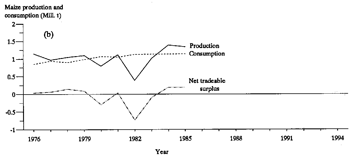
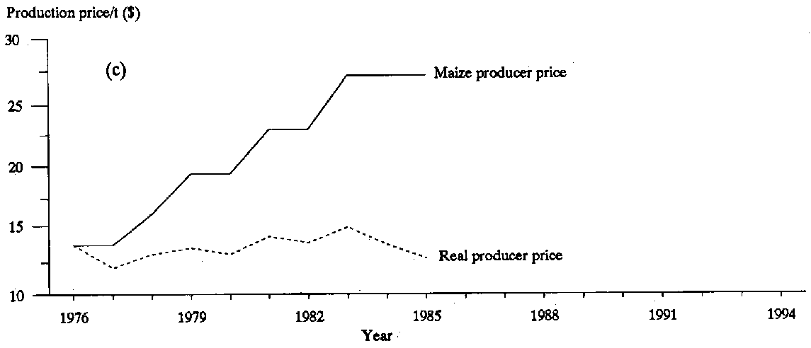
Example: Table 3.10 provides country statistics on disposable income, the consumer price index and population numbers for 1976-95. These are then related to consumption and production data for maize and to producer prices, in order to determine consumption per caput and real producer prices for each year of the period. Figure 3.10 presents the data from Table 3.10 in graphical form.
Exercise: (estimated time required: 4 hours).
Examine Figure 3.10a carefully and compare the graph with the time series data given in Table 3.10. In the graph, a trend line has been drawn by hand for deflated disposable income, forecasted estimates of which have been extrapolated for 1990 and 1995. These estimates have also been entered in the table.
Table 3.10. Derivation of real producer prices and per caput consumption of maize, 1976-95.
Question 1. On Figure 3.10b, draw trend lines for maize production and consumption, and extrapolate values for 1990 and 1995. Enter these values in the table.Question 2. On a separate sheet, derive and plot consumption per caput and extrapolate its trend to 1990 and 1995.
Question 3. On Figure 3.10c, draw the trend line for real producer price and enter your estimates in the table.
Question 4. Identify and comment on any observed and logical relationships between the variables graphed in Figures 3.10a-3.10c. Discuss the relationships between price, income and quantity trends. Indicate whether the country is moving towards being self-sufficient, a net importer or a net exporter of maize.
Question 5. Table 3.11 presents information on production, consumption and producer prices for beef and whole milk. The table is incomplete, and information from Table 3.10 on population and the consumer price index is needed to fill in the blank rows.
· For both products, complete all rows in the table.· Graph the results, as in the previous example.
· Sketch the trend line for each variable and project this to the year 1995. Enter these estimates in Table 3.11.
· For both products, comment on any relationships which you consider logically explainable.
· For both products, determine whether the country is likely to be self-sufficient, a net exporter or a net importer by 1990.
· Why do you think the positive relationship between deflated disposable income per caput and consumption per caput is so strong for all three products? Estimate the implied income elasticity of demand for each product, assuming for this rough estimate that prices and other factors do not influence demand.
Table 3.11. Production. consumption and producer prices of beef and whole milk, 1976-95.
Exercise 3.9: Group Exercise: Production systems, supply and demand. Read the relevant sections of the central case study.
Question 1. Describe the role of beef cattle in the economy of Alphabeta, giving reasons for the changing contribution of the livestock subsector to GDP earnings since independence. Cite statistical data to support your description, where possible.Question 2. Describe quantitatively changes in beef herd growth, offtake rates, urban demand, marketed supply and exports in Alphabeta for the period since independence. Plot past trends in these variables and extrapolate these trends for five years beyond the final year of your data set. Discuss the implications of the extrapolations you have made.
Question 3. What factors have influenced the stability of the beef sector's contribution to the economy of Alphabeta?
Question 4. Describe the main features of Alphabeta's various beef production systems. If possible, indicate the degree of commercialisation in each. Also examine the evidence for changing ownership patterns and land access rights in the communal areas since independence. Comment on the results you obtain. Give quantitative evidence for the significance of each system to the Alphabeta meat industry.
|
Important points (3.7) · Two rough methods of forecasting future production and/or consumption for a particular product are: - analysis of past trends · A rough analysis of a trend is made from time series data in three ways, namely, - by calculating moving averages · Extrapolation can be done by using the changes in the variable over time, moving averages or the average rate of change observed in the past. · Forecast by trend extrapolation method, based on past trends, must be modified for special factors having influence for the future. · Future population and income provide the basis for forecasting demand of a commodity instead of its price. |
![]()
![]()
![]()
