8. TOPOGRAPHICAL SURVEYS - DIRECT LEVELLING
8.0 Introduction
|
| 1. In Chapters 5 and 6, you learned about various devices
for measuring height differences. You also learned how to use these devices
to solve three types of
problems in measuring height differences, which you may face when you
plan and develop a fish-farm (see Section 5.0). Now, you will learn how
to plan surveys to solve these problems, how to record
the measurements you make in your field-book, and how to find
the information you need from these measurements. |
|
|
| |
|
|
What are elevation and altitude?
|
|
2. You have learned what the height of a ground point is. Now, however,
you will need to know a more accurate definition of this term.
- When the height of a point is its vertical distance above or
below the surface of a reference plane* you have selected,
it is called the elevation* of that point.
- When the height of a point is its vertical distance above or
below mean sea level (as the reference plane), it is called the
altitude* of the point.
|
Example
|
|
Elevation of a point above a selected ground
mark A
Altitude of the same point above mean sea level (amsl) |
1.83 m
345 m
|
3. The vertical distance between two points is called the difference
in elevation , which is similar to what you have learned
as the difference in height (see Section 5.0). The process of measuring
differences in elevation is called levelling , and
is a basic operation in topographical surveys.
|
|
|
| |
|
|
|
What are the main levelling methods?
|
|
4. You can level by using different methods, such as:
- direct levelling, where you measure differences
in elevation directly. This is the most commonly used method;
- indirect levelling, where you calculate differences in
elevation from measured slopes and horizontal distances.
|
|
Direct levelling
|
| |
|
|
|
You have already learned about indirect levelling in Section 5.0, when
you learned to calculate differences in elevation
from slopes or from vertical angles.
Now you will learn about direct levelling.

|
|
Indirect levelling
|
What are the kinds of direct levelling?
5. By direct levelling, you can measure both the elevation of points and the
differences in elevation between points, using a level and a levelling
staff (see Chapter 5). There are two kinds of direct levelling:
- differential levelling; and
- profile levelling.
6. In differential levelling , you find the difference in elevation
of points which are some distance apart (see Section 8.1). In the simplest kind
of direct levelling, you would survey only two points A and B from one central
station LS. But you may need to find the difference in elevation between:
- either several points A, B, ... E, surveyed from a single levelling station
LS; or
- several points A ... F, surveyed from a series of levelling stations LS1
... LS6, for example:
7. In profile levelling , you find the elevations of
points placed at short measured intervals along a known line, such as the centre-line
of a water supply canal or the lengthwise axis of a valley. You find elevations
for cross-sections with a similar kind of survey (see Section 8.2).
8. You can also use direct levelling to determine elevations for contour
surveying (see Section 8.3), and for setting
graded lines of slope(see Section 6.9), where you need to combine both differential
levelling and profile levelling.
|
Differential levelling
|
|
Profile levelling
|
9. There are several simple ways to determine the elevations of ground points
and the differences in elevation between ground points. You will use a level and
a levelling staff with these methods. In the following sections, each method is
fully described to help you choose between them. Table
10 will also help you to compare the various methods and to select the one
best suited to your needs in each type of situation you may encounter.
|
TABLE
10
Direct levelling methods
|
Section
|
Type
|
Method
|
Suitability
|
Remarks
|
|
|
Differential levelling
|
Open traverse
|
Long, narrow stretch of land
|
Check for closing error
|
|
|
Differential levelling
|
Closed traverse
|
Perimeter of land area and base line for radiation
|
Check for closing error.
Combine with radiating
|
|
|
Differential levelling
|
Square-grid
|
Small area with little vegetation
|
Squares 10 to 20 m and 30 to 50 m
|
|
|
Differential levelling
|
Radiating
|
Large area with visibility
|
Combined with closed traverse
|
|
|
Longitudinal profile levelling
|
Open traverse
|
Non-sighting and sighting level
|
Check for closing error
|
|
|
Cross-section profile levelling
|
Radiating
|
Sighting level with visibility
|
|
|
|
Contouring
|
Direct
|
Detailed mapping of small area with a sighting
or a non-sighting level and target levelling staff
|
Slow and accurate.
Progress uphill
|
|
|
Contouring
|
Square-grid
|
Small area with little vegetation Especially
if perimeter has been surveyed. Small to medium scale mapping
|
Terrain, scale and accuracy depend on contour
interval.
Progress uphill.
Suitable for plane-tabling
|
|
|
Contouring
|
Radiating
|
Small to medium scale mapping of large area
|
Fast and fairly inaccurate. Progress uphill.
Suitable for plane-tabling
|
|
|
Contouring
|
Cross-sections
|
Preliminary survey of a long and narrow stretch
of land
|
Fast, fairly inaccurate. Progress uphill.
Suitable for plane-tabling
|
|
8.1 How to level by differential
|
What is differential levelling?
|
|
1. You can best understand differential levelling by first considering
only two points, A and B , both of which
you can see from one central levelling station, LS .
- Sight with a level from LS at the levelling staff on point A. The
point where the line of sight meets the levelling staff is point X.
Measure AX. This is called a backsight (BS).
|
|
Find AX with a backsight
|
| |
|
|
- Turn around and sight from LS at the levelling staff on point B. The
point where the line of sight meets the levelling staff is point Y.
Measure BY. This is called a foresight (FS).
|
|
Find BY with a foresight
|
| |
|
|
- The difference in elevation between point A and point B
equals BC or (AX- BY) or (backsight BS - foresight FS).
|
|
The difference in elevation between
points A and B equals AX minus BY
|
| |
|
|
|
- If you know the elevation of A, called E(A), you can calculate
the elevation of B, called E(B), as BS -FS + E(A).
- But BS + E(A) = HI, the height of the instrument or
the elevation of the line of sight directed from the level.
|
|
|
| |
|
|
(the elevation at point B being equal to the height of the levelling
instrument, minus the foresight).
|
|
|
What are backsights and foresights?
|
|
It is important for you to understand exactly what "backsight"
and "foresight" are in direct levelling.
2. A backsight (BS) is a sight taken with
the level to a point X of known elevation E(X), so that the
height of the instrument HI can be found. A backsight in direct levelling
is usually taken in a backward direction, but not always. Backsights are
also called plus sights (+ S), because you must always add
them to a known elevation to find HI.
|
|
|
| |
|
|
|
3. A foresight FS is also a sight taken
with the level, but it can be on any point Y of the sight line
where you have to determine the elevation E(Y). You will usually take
it in a forward direction, but not always. Foresights are also called
minus sights (-S) , because they are always subtracted
from HI to obtain the elevation E of the point. Remember:
|
|
|
| |
|
|
Surveying two points with one turning point
|
| 4. Often you will not be able to see at the same time the
two points you are surveying, or they might be far apart. In such cases,
you will need to do a series of differential levellings
. These are similar to the type explained above, except that you will
use intermediate temporary points called turning points (TP).
|
|
|
| |
|
|
| 5. You know the elevation of point A, E(A) = 100 m, and you
want to find the elevation of point B, E(B), which is not visible from a
central levelling station. Choose a turning point C about halfway
between A and B. Then, set up the level at LS1, about halfway between A
and C. |
|
|
| |
|
|
| 6. Measure a backsight on A (for example, BS = 1.89 m). Measure
on C a foresight FS = 0.72 m. Calculate HI = BS + E(A) = 1.89
m + 100 m = 101.89 m. Find the elevation of turning point C as E(C)
= HI-FS = 101.89 m - 0.72 m = 101.17 m. |
|
|
| |
|
|
| |
|
|
|
7. Move to a second levelling station, LS2, about halfway between C and
B. Set up the level and measure BS = 1.96 m, and then FS = 0.87 m. Calculate
HI = BS + E(C) = 1.96 m + 101.17 m = 103.13 m. 0btain E(B)
= HI- FS = 103.13 m - 0.87 m = 102.26 m.
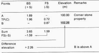
8. You can make the calculations more easily if you record the field
measurements in a table , as shown in the example. You
will not make any intermediate calculations. All BS's and all FS's must
be added separately. The sum FS is subtracted from the sum BS to find
the difference in elevation from point A to point B.
- A positive difference means that B is at a higher elevation
than A.
- A negative difference means that B is at a lower elevation
than A.
|
|
|
| |
|
|
|
Knowing the elevation of A, you can now easily calculate the elevation
of B. In this case, E(B) = 100 m + 2.26 m = 102.26 m; this is the same
as the result in step 7, which required more complicated calculations.
This kind of calculation is called an arithmetic check.
Example
Table form for differential levelling with one turning point.
|
|
|
Surveying two points using several turning points
9. Often you will need to use more than one turning point between a point of
known elevation and another point of unknown elevation. To do this, you can
use the procedure you have just learned, but you will need to record
the field measurements in a table to make calculating the results
easier.
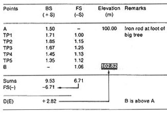
10. Knowing the elevation of point A, you need to find the elevation
of B. To do this, you need for example five turning points
, TP1 ... TP5, and six levelling stations, LS1 ... LS6.
Note : the turning points and the levelling stations
do not have to be on a straight line, but try to place each levelling
station about halfway between the two points you need to survey from
it.
11. From each levelling station, measure a backsight (BS)
and a foresight (FS) , except:
- at starting point A, where you have only a backsight
measurement.
- at ending point B, where you have only a foresight
measurement.
|

|
| |
|
Example
Table form for differential levelling with several turning points.
|
Using step 8 as a guideline, enter all measurements in a table and calculate
the results as shown in the example below. You will find that point B is 2.82
m higher than point A and, therefore, that its elevation is E(B) = 100 m + 2.82
m = 102.82 m.
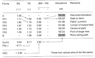
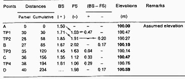
12. Even if you are careful, you may still make mistakes when you make your
arithmetic calculations from the table. To reduce this kind of error, add two
additional columns to your table that will make checking your calculations
easy. In these columns, enter the difference (BS- FS), either positive (+ )
or negative (-), between the measurements you took at each levelling station.
For example, from LS1 you measure BS (A) = 1.50 m and FS (TP1) = 1.00 m. The
difference 1.50 m- 1.00 m = 0.50 m is positive, and you enter it in the (+)
column on the TP1 line.
The arithmetic sum of these differences should be equal to the calculated
difference in elevation D(E) = +2.82 m. These columns will also help you to
calculate the elevation of each turning point , and to check
on the elevation of point B more carefully.
|
Example
Differential levelling with several turning points
|
|
Making topographical surveys by straight open traverses
|
|
13. By now, you have learned enough to make a topographical survey of
two distant points by measuring the horizontal distance between them and
the difference in their elevation.
When you survey a future fish-farm site, you will use a very similar
method. You can then prepare a topographic map of the site (see Chapter
9), which will become a useful guide for designing the fish-farm.
14. This is a survey method using straight open traverses
, that is, several intermediate stations along one straight line.
You know for example the elevation of starting point A, E(A) = 63.55 m.
You want to know the distance of point B from point A, and its elevation.
Because of the type of terrain on which you are surveying, you cannot
see point B from point A, and you need two turning points
, TP1 and TP2 , for levelling. Measure horizontal distances
as you move forward with the level, from point A toward point B; try to
progress along a straight line. If you cannot, you will need to use the
broken open traverse survey method, which involves measuring the
azimuths of the traverse sections as you move forward and change direction
(see step 17).
|
|
|
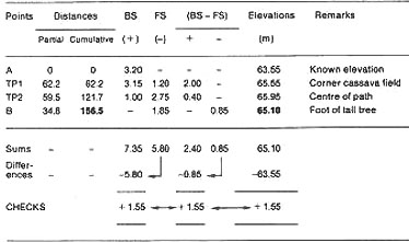
15. Set out a table like the one in step 12, and add two columns
to it for horizontal distances. Enter all your distance and height measurements
in the main part of the table. Then, in the first additional column, record
each partial distance you measure from one point to the next one.
In the second column, note the cumulated distance , which is the
distance calculated from the starting point A to the point where you are measuring.
The last number in the second column will be total distance AB.
|
Example
Topographical survey of a straight open traverse by differential
levelling
|
16. Conclusions . Point B is 1.55 m higher than A and its elevation
is 65.10 m. It is 156.5 m distant from point A. The arithmetic check from the
(BS- FS) differences agrees with the calculated difference in elevation.
Making topographical surveys by broken open traverses
|
| 17. Remember, that if you survey by broken open traverses
(or zigzags), you will also have to measure the azimuth of each traverse section as you
proceed, in addition to distances and elevations. |
|
|
| |
|
|
|
18. You need for example to survey open traverse ABCDE from known point
A. You require four turning points, TP1, TP2, TP3 and TP4. You want to
know:
- the elevations of points B, C, D and E;
- the horizontal distances between these points;
- the position of each point in relation to the others, which will help
you in mapping them.
|
|
|
| |
|
|
|
|
| Proceed with the differential levelling as described earlier,
measuring foresights and backsights from each levelling
station. Measure azimuths and horizontal distances as you progress from
the known point A toward the end point E. All the azimuths of the turning
points of a single line should be the same. This will help you check your
work. |
|
|
| |
|
|
| 19. Make a table similar to the one shown in step
15, and add three extra columns to it for recording
and checking the azimuth values. Enter all your measurements
in this table. At the bottom of the table, make all the checks on the elevation
calculations, as you have learned to do them in the preceding steps. |
|
|
| |
|
|
|
Example
Topographical survey of a broken open traverse by
differential levelling
|
Checking on levelling errors
|
| 20. Checking on the arithmetic calculations does not tell
you how accurate your survey has been. To fully check on your accuracy,
level in the opposite direction , from the final point to the
starting point, using the same procedure as before. You will probably find
that the elevation of point A you obtain from this second levelling differs
from the known elevation. This difference is the closing error
. |
|
|
| |
|
|
|
Example
From point A of a known elevation, survey by traversing through
five turning points, TP1 ... TP5, and find the elevation of point B. To
check on the levelling error, survey by traversing BA through four other
turning points, TP6 ... TP9; then calculate the elevation of A. If the
known elevation of starting point A is 153 m, and the calculated elevation
of A at the end of the survey is 153.2 m, the closing error is 153.2 m
- 153 m = 0.2 m.
|
|
|
| |
|
|
| |
|
|
21. The closing error must be less than the permissible error, which is the
limit of error you can have in a survey for it to be considered accurate. The
size of the permissible error depends on the type of survey (reconnaissance,
preliminary, detailed, etc.) and on the total distance travelled
during the survey. To help you find out how accurate your survey has been, calculate
the maximum permissible error (MPE) expressed in
centimetres , as follows:
|
Reconnaissance and preliminary surveys:
MPE(cm) = 10ÖD
Most engineering
work:
MPE(cm) = 2.5ÖD
|
where D is the distance surveyed, expressed in kilometres
.
Example
You have just finished a reconnaissance survey. Your closing error was
0.2 m or 20 cm, at the closure of a traverse 2.5 km + 1.8 km = 4.3 km long.
In this case, the maximum permissible error (in centimetres) equals 10Ö4.3
= 10 x 2.07 = 20.7 cm. Since your closing error is smaller than the MPE, your
levelling measurements have been accurate enough for the purposes of a reconnaissance
survey.
Making topographical surveys by closed traverses
|
| 22. In the previous section, you made a topographical survey
along an open traverse joining points A and B. You can survey a closed
traverse , such as the perimeter of a fish-farm site, in a similar
way. You should use each perimeter summit A, B, C, D, E and F
of the polygon as a survey point, and plot turning points between these
summits as you need to. Make a plan survey as
explained in Section 7.1, and use differential levelling to find the
elevation of each perimeter point.
23. If you do not know the exact elevation of starting point A, you can
assume its elevation, for example E (A) = 100 m. Start the survey
at point A , and proceed clockwise along the perimeter
of the area. Take levelling staff readings at TP1, TP2, B, TP3, etc.,
until you reach starting point A again and close the traverse. At the
same time, make any necessary horizontal distance and azimuth measurements.
Record your measurements either in two separate tables , one
for plan surveying and one for levelling, or in one table which
includes distance measurements. From the (BS-FS) columns, you can easily
find the elevation of each point on the basis of the known (or assumed)
elevation at point A. Make all the checks on the calculations
as shown in steps 15 and 16. Find the closing levelling error at point
A (see step 20). This error should not be greater than the maximum
permissible error (see step 21).
|
|
|
| |
|
|
|
Example
Topographical survey of a closed traverse by differential
levelling
|
|
|
|
Making topographical surveys
by the square grid
|
|
|
|
24. The square-grid method is particularly useful for surveying small
land areas with little vegetation. In large areas with high vegetation
or forests, the method is not as easy or practical. To use the method,
you will lay out squares in the area you are surveying, and determine
the elevation of each square corner.
25. The size of the squares you lay out depends
on the accuracy you need. For greater accuracy, the sides of the squares
should be 10 to 20 m long. For reconnaissance surveys, where you do not
need to be as accurate, the sides of the squares can be 30 to 50 m long.
|
|
|
| |
|
|
| 26. In the field choose base line AA and clearly
mark it with ranging poles. This base line should preferably be located
at the centre of the site, and it should be parallel to the longest side
of the site. When you work with a compass, you may find that it helps to
orient this base line following the north-south direction.
27. Working uphill, chain along this baseline from the perimeter of the
area, and set stakes at intervals equal to the size you have
chosen for the squares, such as 20 m. Clearly number these stakes 1, 2,
3, . . . n.
|
|
|
| |
|
|
| 28. From each of these stakes, lay out a line, perpendicular to the base line
, that runs all the way across the site. |
|
|
29. Proceed by chaining along the
entire length of each of these perpendiculars, on either side of
the base line . Set a stake every 20 m (the selected square size).
Identify each of these stakes by:
- a letter (A, B, C, etc.) which refers to the
line, running parallel to the base line, to which the point belongs;
- a number (1, 2, 3.... n) which refers to the perpendicular,
laid out from the base line, to which the point belongs.
Example
20 m from point A1, perpendicular 2 crosses line AA at point
A2.
20 m to the left of point A2 lies point B2 , on line BB.
|
|
|
| |
|
|
|
30. Now that you have laid out the square grid on the ground,
you need to find the elevation of each corner of the squares
, which you have marked with stakes. First establish a bench-mark (BM) on base line
AA near the boundary of the area and preferably in the part with
the lowest elevation (see steps 42-44). This bench-mark can be either
at a known elevation (such as one point on a previously surveyed
traverse), or at an assumed elevation (such as 100
m) (see step 45).
31. You will level the square grid points in two stages.
- Starting from the bench-mark, measure the differences in elevation
for all the base points A1, A2, A3, ... An. This is called
longitudinal profile levelling (see Section
8.2).
- Then, starting at these base-line points with known elevations, measure
the differences in elevation for all points of each of the perpendiculars,
on each side of the base line (for example, B2, C2 and D2 followed by
E2, F2 and G2). This is called cross-section
levelling (see Section 8.2).
|
|
|
| |
|
|
| 32. If you use a sighting level you
can make a radiating survey (see step 34). Set up your level
at LS1 and take a backsight reading on the bench-mark (BM). Then, take foresight
readings on as many base-line points as possible. From this, find the height
of the instrument (HI) and point elevations, with HI = E(BM) + BS and E
(point) = HI- FS. When necessary, change the levelling station and find
a new HI on the last known point, which is used as a turning point. Then
measure a series of foresights. Since the distances of the square grid are
all fixed, you do not need to measure them any more. Note down your measurements
in a table, as shown in the example. |
|
|
| |
|
|
|
Example
Topographical survey by square grid with a sighting
level
|
Levelling station
|
Point
|
BS
|
HI
|
FS
|
Elevation
|
Remarks
|
|
1
|
BM
|
1.53
|
101.53
|
-
|
100.00
|
Assumed elevation
|
| |
A1
|
-
|
101.53
|
1.25
|
100.28
|
|
| |
A2
|
-
|
101.53
|
1.20
|
100.33
|
|
| |
A3
|
-
|
101.53
|
1.15
|
100.38
|
|
|
2
|
A3
|
1.48
|
101.86
|
-
|
100.38
|
Turning point
|
| |
A4
|
-
|
101.86
|
1.41
|
100.45
|
|
| |
...
|
...
|
...
|
...
|
...
|
|
| |
A9
|
...
|
...
|
...
|
...
|
|
|
5
|
A1
|
1.20
|
101.48
|
-
|
100.28
|
Known from A1 above
|
| |
B1
|
-
|
101.48
|
0.23
|
100.25
|
|
| |
C1
|
-
|
101.48
|
0.25
|
100.23
|
|
| |
D1
|
-
|
101.48
|
0.28
|
100.20
|
|
|
6
|
D1
|
1.30
|
101.50
|
-
|
100.20
|
Turning point
|
| |
E1
|
-
|
101.50
|
0.35
|
100.15
|
|
| |
...
|
...
|
...
|
...
|
...
|
|
| |
G1
|
-
|
101.50
|
0.47
|
100.03
|
|
|
9
|
A2
|
1.35
|
101.68
|
-
|
100.33
|
Known from A2 above
|
| |
B2
|
...
|
...
|
-
|
...
|
|
| |
...
|
...
|
...
|
...
|
...
|
|
|
12
|
F2
|
...
|
...
|
-
|
...
|
|
| |
G2
|
...
|
...
|
-
|
...
|
|
|
13
|
A3
|
...
|
...
|
-
|
100.38
|
Known from A3 above
|
| |
...
|
...
|
...
|
...
|
...
|
|
|
| |
Example
Topographical survey by square-grid with a
non-sighting level
|
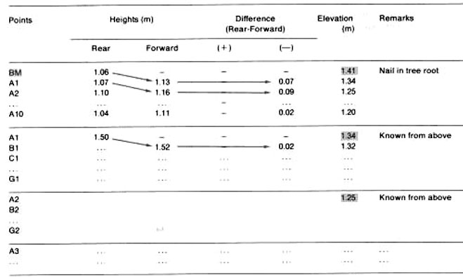
| 33. If you use a non-sighting level , first follow
base line AA. Start with the bench-mark as a reference point, and survey
all its points A1, A2, ... A9. Then, repeat this surveying procedure along
each of the perpendiculars, starting with the known base-line points as
the reference points.
Enter all your measurements in a table, and find the elevation of each
point of the square grid (see steps 38-41 for a further explanation).
You can check calculations and survey measurements at the bottom part
of the table (see this Section, step 41).
|
|
|
Making topographical radiating
surveys
|
|
34. When you make a radiating survey (see Section 7.2), you first need
to determine the height of the instrument HI at
levelling station 0. Sight at a point X of known elevation E(X), and find
a backsight (BS). Then,
35. Then you need to find the elevation of each of the points A, B, C
and D. Sight at each of them in turn. You will find a foresight (FS)
for each. Calculate their elevations as
36. Record all your measurements in a table. This table may also include
plan-surveying information, such as azimuths and horizontal distances.
You might also use two different tables as explained in step 23. The first
line of the table will refer to the known point X .
This point can be one of the perimeter points which you have already determined,
or it can be a benchmark (see step 42).
You find the position of point 0 from the azimuth of line OX
and the horizontal distance OX.
|
|
Use X as a point of reference
|
| |
|
|
|
|
| |
|
|
|
Example
Topographical radiating survey
|
Levelling station
|
Point
|
BS (m)
|
HI (m)
|
FS (m)
|
Elevation (m)
|
Azimuth (degree)
|
Distance (m)
|
Remarks
|
|
0
|
X
|
0.45
|
144.00
|
-
|
143.55
|
285
|
35.3
|
Known elevation |
|
0
|
A
|
-
|
144.00
|
1.65
|
142.35
|
50
|
29.6
|
|
|
0
|
B
|
-
|
144.00
|
0.97
|
143.03
|
131
|
27.3
|
|
|
0
|
C
|
-
|
144.00
|
0.60
|
143.40
|
193
|
25.1
|
|
|
0
|
D
|
-
|
144.00
|
1.12
|
142.88
|
266
|
24.8
|
|
|
Combining traversing and composite radiating
|
37. This method combines radiating with a closed traverse.
You can use it to gather the information you need to make a topographical
map of a land area such as a fish- farm site (see Chapter
9). Using what you have learned so far about surveying, do the following:
(a) With a closed traverse, plan survey the boundaries
of the area ABCDEA. Find the lengths and directions of all of its sides
(see Section 7.1). |
|
Fix the position of LS 1 
|
| |
|
|
| (b) In the interior of the site, choose a series of levelling
stations 1, 2, 3.... 6, from which you can survey the surrounding
area by radiating. |
|
Choose levelling stations
|
| |
|
|
| (c) Fix the position of levelling station 1 by
measuring it in relation to known boundary points such as A and B. You can
use the plane-tabling and triangulation methods
(see Section 9.2). |
|
Survey the boundaries
|
| (d) Join all the selected levelling stations by straight lines
to form a closed traverse . Survey it, using turning points as
necessary, to fix the position of each station and to determine
its elevation . Check for the closing error (see Section 7.1)
and this section, step 20). |
|
Survey all the levelling stations
|
| |
|
|
|
(e) Now you are ready to start the detailed topographical survey, proceeding
from each known levelling station in turn. From station 1, set up a series
of radiating straight lines at a fixed-angle interval (such
as 20°). This means that each radiating line will be 20° from the next.
Use your magnetic compass and ranging poles or stakes. Mark on the ground
the north-south line. You will call this the zero-degree
line . Standing on this line at station 1, measure and
mark a line with a 20° azimuth. Then, moving around in a clockwise direction
on the same point, measure and mark in turn lines with azimuth 40°, 60°,
... 340°.
Note: the fixed-angle interval you use depends on how accurate
a survey you need. Smaller angles will help you make a more accurate map
of the site.
|
|
Mark radiating lines at the interval you have chosen
|
| |
|
|
| (f) Start at Station 1, using differential levelling
, to survey ground points on each of these radiating lines. You may choose
any points you want to measure, for example the intersection of the radiating
line with the boundary of the site, or a point where the ground changes
slope suddenly, or the location of a rock or tree. Besides finding the
elevation of these points, measure the distance between
each point and the levelling station, so that you will be able to map them
later on. |
|
|
| |
|
|
| (g) Move to each levelling station in turn (2, 3, 4, 5, 6),
and repeat steps (e) and (f), measuring the elevation and distance of unknown
random points along the radiating lines -, so as to survey the whole
area. |
|
|
| |
|
|
|
(h) Record all the measurements in a table, and calculate the elevations
of all the surveyed points (see this section, step 36). You will need
two additional columns in this table:
- one column marked "Line" , where you will record
the azimuth of each line;
|
|
|
| |
|
|
- one column marked "Cumulative distances"
. In this space, you can separately calculate
the distance from the levelling station to the points surveyed for each
line.
|
|
|
| |
|
|
|
Example
Topographical survey of partial area by composite
radiating
|
Making topographical surveys with non-sighting levels
|
|
38. You can also make topographical surveys along straight lines by using
non-sighting levels , such as the line
level (see Section 5.2) or the flexible-tube water level (see Section 5.3). You
have already learned how to measure height differences by using the square-grid
method with such levels (see this section, step 33).
Remember , when you lay out your grid, that the
distance between points cannot be more than the length of your level.
|
|
|
| |
|
|
| 39. Work in a team of two or three with this method. Both
the rear person and the front person will take measurements
in the field, but only one person should be responsible for noting
down these measurements in the field book. |
|
|
|
|
| |
|
Example
Topographical survey with a line level (20 m)
|
40. Record the measurements in a table for each levelled section. You will
be measuring horizontal distances from one point to the next, and
differences in elevation between one point and the next. At both the starting
point and the last point, there is only one height measurement. The rear person
will measure it on the starting point, and the front person will measure it
on the last point.
41. Find the cumulated distances from the starting
point and the elevations of each point, as shown in the example.
There are three possible checks , which you make
at the bottom part of the table.
Making
bench-marks for topographical surveys
42. As you have just learned, you will always start differential levelling
surveys by measuring a height on a ground point of known or assumed
elevation . This point becomes a bench-mark (BM)
. The elevation of this bench-mark will form the basis for finding the elevation
of the other points you need to survey in the area.
43. A bench-mark should be permanent . You should always
establish at least one bench-mark near the construction site of a fish-farm
to act as a fixed reference point or object. You may also use a bench-mark as
a turning point during topographical surveys.
44. A bench-mark should be a very well-defined point
. You should be able to find and recognize it easily. It should be easy to reach,
so that you can hold a levelling staff on it. You can establish a bench-mark:
- on wooden or bamboo stakes set
near the construction site;
- by driving a nail into a tree or
tree stump, near the ground line, where it will remain even when the tree is cut down;
- by fixing a piece of iron rod in
a concrete block near ground level;
- on permanent objects or
structures which are unlikely to settle, move or be disturbed, such as a bridge, a large
rock or the wall of a building.
Note : it is best to paint the bench-mark, or set several
signs near it, to show its location.
|
|
|
|
| |
|
|
|
|
|
|
| |
|
|
| 45. Generally, the elevation of a bench-mark E(BM) is
not known but is assumed . When you have established the first bench-mark
for a building project, you give it an elevation that is a convenient
whole number , such as 100 m. The number you choose should
be large enough to prevent any point in the surveyed area from having a
negative elevation.
Note : you have seen in previous examples that
some surveys are related to previously surveyed points, This means that
the measurements in the survey are based on these points. These points
then become turning-point bench-marks . You find
their elevations by levelling, and these then become known elevations.
|
|
|
8.2 How to level by profile
|
What is the purpose of profile levelling?
|
| 1. The purpose of profile levelling is to determine the changes
in the elevation of the ground surface along a definite line
. (You have already learned about profile levelling used with the square-grid
method in Section 8.1, step 31.) This definite line AB might be the centre-line
of a water-supply canal, a drainage ditch, a reservoir dam, or a pond dike.
This line might also be the path of a river bed through a valley, where
you are looking for a dam site, or it might be one of several lines, perpendicular
to a river bed, which you lay out across a valley when you are surveying
for a suitable fish-farm site. |
|
Ground line AB
|
| |
|
|
| 2. You will usually transfer the measurements you obtain during
profile levelling onto paper, to make a kind of diagram or picture called
a graph . This will show changes in elevation, and how they are
related to horizontal distances. This kind of graph is called a
ground profile. You will learn how to make one in Sections 9.5 and 9.6. |
|
Profile AB
|
What does profile levelling
consist of?
|
|
3. When you profile level, you are determining a series of elevations
of points which are located at short measured intervals along a fixed
line . These elevations determine the profile of the line.
4. There are two kinds of profiles which are commonly used in fish culture:
longitudinal and cross-section profiles.
|
|
|
| |
|
|
- You usually survey cross-section profiles along
a line which is perpendicular to a surveyed longitudinal profile,
using its points of known elevation as bench-marks. Cross-sections of
valleys are useful in helping you locate a good fish-farm site. On a
smaller scale, you can also survey cross-sections for water-supply canals,
for dam construction, and for pond construction. You have already learned
how to use cross-section profiles when surveying by the square-grid
method (see Section 8.1, step 31).
|
|
|
|
8. When you need to move the level to a new station so that you can take
readings on the points ahead:
- first, choose a turning point TP and take a foresight FS
to find its elevation from LS1;
- move to the next levelling station LS2, from which you can see the
turning point TP;
- take a backsight BS on this turning point to find the new height
of the instrument HI.
|
|
Take a foresight from LS 1 to the turning point
|
| |
|
|
| 9. Read foresights FS on as many points as possible until
you reach the end point of AB. If necessary, use another turning point and
a new levelling station as described in step 8. |
|
Take a backsight from LS 2 to the turning point
|
| |
|
|
| 10. Note down all your measurements in a field book, using
a table similar to the ones you have used with other methods. Find the elevations
of the points (except for the turning point) by subtracting each FS from
its corresponding HI. In the example of the table shown here, cumulated
horizontal distances (in metres) appear as point numbers 00, 25, 50, 65,
etc. in the first column. |
|
Take foresights at the points you have marked
|
| |
|
|
|
Example
Longitudinal profile levelling with a sighting level
in a radiating survey
|
Points(m)
|
BS
|
HI
|
FS
|
Elevation(m)
|
Remarks
|
|
BM
|
1.37
|
2.87
|
-
|
1.50
|
Nail at foot of tree stump |
|
00
|
-
|
2.87
|
1.53
|
1.34
|
Beginning of canal |
|
25
|
-
|
2.87
|
1.67
|
1.20
|
|
|
50
|
-
|
2.87
|
1.73
|
1.14
|
|
|
65
|
-
|
2.87
|
1.90
|
0.97
|
Marked change of slope |
|
75
|
-
|
2.87
|
2.05
|
0.82
|
|
|
100
|
-
|
2.87
|
2.22
|
0.65
|
|
|
TP
|
1.80
|
3.07
|
1.60
|
1.27
|
On stone |
|
125
|
-
|
3.07
|
2.27
|
0.80
|
|
|
150
|
-
|
3.07
|
2.37
|
0.70
|
|
|
175
|
-
|
3.07
|
2.57
|
0.50
|
|
|
200
|
-
|
3.07
|
2.77
|
0.30
|
|
|
230
|
-
|
3.07
|
3.00
|
0.07
|
End of canal |
|
Longitudinal profile levelling by traversing
|
|
11. You need to survey the same line AB, the centre-line of a water canal,
for profile levelling. You will use a non-sighting level, such as the flexible tube water
level (see Section 5.3). Since you are using this kind of level, you
will survey by traversing. Mark the line AB with stakes driven
into the ground at regular intervals. The length of these intervals depends
on the working length of your level (in this case, 10 m). Where there
are marked changes in slope, add intermediate stakes. On each stake, mark
its distance from the initial point A.
12. Level a tie-in line between bench-mark
BM and the initial point A (see Section
5.3, steps 6-12). This will give you the elevation of point A, through
intermediate point 1.
|
|
Mark the line at 10-m intervals
|
| |
|
|
|
13. Proceed with the levelling of the marked points along
the line, using this method. At each point, you will make two scale readings,
one rear and one forward, except at the final point where you will take
only one height measurement.
14. One person should be responsible for recording the measurements
in a field book, using a table similar to the one in Section 8.1, step
41. But, in this case, you will not need to enter the distances in the
table, since they identify the surveyed points. Checks are made at the
bottom of the table as usual. Remember that in this type of survey there
is no need for turning points.
|
|
Level a tie-in from the bench-mark,
then level the points on the line
|
| |
|
|
|
Example
Longitudinal profile levelling by traversing with
a flexible tube water level (10 m)
|
Cross-section profile levelling
|
15. After you have found the elevations of points along a longitudinal
profile, you can proceed with the survey of perpendicular cross-sections
. These cross-sections can pass through as many of the points as necessary.
Cross-sections are commonly used for contouring long, narrow stretches
of land (see Section 8.3).
16. You will need to have more information on some of the longitudinal
profile points. Choose these points and mark them. Then, set
out and mark perpendicular lines at these points (see Section 3.6),
and extend these perpendiculars on both sides of the traverse
as far as you need to. In this type of levelling, such perpendiculars
are called the cross-section lines .
|
|
|
| |
|
|
| Note : at points where the traverse
changes direction (for example, at point 175 in the drawing), you should
set out two perpendicular lines E and F; each line will be perpendicular
to one of the traverse sections. |
|
At a turn, make two cross-sections
|
| |
|
|
|
17. Choose and clearly mark the points you want to survey on each cross-section
line. In this case, these points do not have to be regularly spaced. Rather,
they should be at places where the terrain changes since they
should mark changes in slope.
18. As you know the elevations of the traverse points from a previous
survey, you may treat these points as bench-marks. Proceed with the profile
levelling of selected points along the cross-section lines as explained
earlier. You may survey them:
Note : you can also survey by traversing using a simple sighting level such as
a bamboo sighting level (see Section 5.6) or a hand level (see Section
5.7).
|
|
|
19. Your field notes will be similar to those shown in either
step 10 or 14, depending on the levelling method you use. You will identify
the points differently, however. You identify each cross-section line by
the number of the traverse point of known elevation. To do this,
identify the surveyed points along each cross-section line according to whether
they are to the left or the right of the traverse . Also use
their distance (in metres) from the traverse points as identification. The following
example is of field notes and calculations for a radiating survey, where each
cross-section was surveyed from a single levelling station.
|
Example
Cross-section profile levelling by radiating
|
Traverse Point
|
Point
|
BS(m)
|
HI(m)
|
FS(m)
|
Elevation(m)
|
Remarks
|
| |
Left
|
Right
|
|
|
|
|
|
|
50
|
...
|
...
|
...
|
...
|
...
|
...
|
|
|
75
|
-
|
-
|
0.54
|
40.94
|
-
|
40.40
|
Edge of existing path
|
| |
10
|
-
|
|
40.94
|
1.09
|
39.85
|
|
| |
18
|
-
|
|
40.94
|
1.15
|
39.79
|
|
| |
-
|
9
|
|
40.94
|
0.85
|
40.09
|
|
| |
-
|
16
|
|
40.94
|
0.68
|
40.26
|
|
|
100
|
-
|
-
|
1.15
|
38.96
|
-
|
37.81
|
Edge of maize field
|
| |
8
|
-
|
|
38.96
|
1.23
|
37.73
|
|
| |
-
|
4
|
|
38.96
|
1.11
|
37.85
|
|
| |
-
|
16
|
|
38.96
|
0.78
|
38.18
|
|
|
125
|
-
|
-
|
0.97
|
36.64
|
-
|
35.67
|
Edge of small forest
|
| |
5
|
-
|
|
36.64
|
1.12
|
35.52
|
|
| |
20
|
-
|
|
36.64
|
1.55
|
35.09
|
|
| |
-
|
14
|
|
36.64
|
1.03
|
35.61
|
|
| |
|
25
|
|
36.64
|
0.89
|
35.75
|
|
|
150
|
...
|
...
|
...
|
...
|
...
|
...
|
|
|
8.3 How to contour
|
What is a contour?
|
| 1. A contour is an imaginary continuous line or curve which
joins ground points of an equal elevation. The elevation of the ground points
must be measured from the same reference plane*. |
|
|
| |
|
|
|
Example
When you pour water into a hole in the ground, you will see that
the surface of the water forms a continuous line made up of the water's
points of contact with the sides of the hole. This line shows one contour
for this particular water depth in the hole. A lake or a reservoir also
has a surface contour which depends on its water level.
|
|
|
| |
|
|
What is contouring?
|
|
2. Contouring means surveying to identify the contours on
the ground, lay them out with markers, and plot them on a plan or map.
You will learn more about planning and mapping
contours in Section 9.4.
|
|
|
|
3. Contouring is used in fish culture to solve two kinds of problem:
- if you have fixed the location of a point, you may have to identify
the contour passing through that point;
Example
You have chosen the end-point of your water-supply canal on a fish-farm
site. Now you have to identify the canal's centre-line, which usually
follows a contour back to the water source (which may be a point along
a river, or the outlet pipe of a pump).
|
|
|
| |
|
|
|
- If you need to prepare a plan or map showing the ground relief of
an area, you must find out the location of contours on the ground
and be able to transfer them onto paper.
Example
You have chosen a fish-farm site. Before you can plan, design and
build the farm, you will need to make a topographical map showing the
location of a series of contours from which you will be able to define
the ground relief of the site.
|
|
|
| |
|
|
|
4. You have already learned how to
find a contour on the ground from a fixed point, in the sections on
contouring devices (see Sections 6.2-6.8).
5. In the following steps, you will learn how to survey contours
over a land area so that you can prepare a topographical map (see
Section 9.4).
|
|
|
| |
|
|
|
What are the main methods for contouring?
|
|
6. It would be an impossible task to identify all the contours in one
area. Therefore, you will have to decide how many contours you need to
identity in each area. You will have to fix the difference in elevation
between contours which are next to each other. This is called the
contour interval .
7. Choosing which contour interval to use depends mainly on the accuracy
you need, on the scale of the map you will prepare (see Section 9.1) and
on the kind of terrain you are surveying. Contour intervals usually
vary from 0.25 m to 1 m . This range of intervals allows good accuracy,
and makes it possible to produce large-scale topographical maps for flat
or slightly sloping ground (which is usually the type of ground used for
fish-culture sites). Since smaller contour intervals make contouring much
more difficult, you will usually make reconnaissance and preliminary surveys
with a contour interval greater than the one you use for later, more detailed
surveys.
|
|
|
| |
|
|
|
Example
Relationship between the size of contour intervals and various factors
|
Factor
|
Contour intervals
|
|
Smaller
|
Larger
|
| Required accuracy |
High
|
Low
|
| Mapping scale (Section 9.1) |
Large-scale
|
Small-scale
|
| Type of terrain |
Flat
|
Sloping
|
|
|
|
| |
|
|
|
8. There are two main methods of surveying contours:
- a direct method; in which you trace and mark the line of
each contour on the ground, and then plan survey these lines so that
they can be mapped,
- an indirect method; in which you make a topographical survey
of the area to find a series of points of known elevation. Then you
enter them on a map and determine the contours from this map.
|
|
Direct contouring
|
| |
|
|
Selecting the contouring method
|
|
|
|
9. When selecting the method you will use for contouring, remember that:
- the direct method is much slower, but is more accurate.
Use it only to contour a relatively small area which you need to map
in detail, on a large scale;
- the indirect method is faster, but it is not so accurate.
Use it to contour large areas that you will map on a medium or small
scale. It should preferably be combined with plane-tabling
(see Section 7.5).
|
|
Indirect contouring
|
Laying out contours on the ground
with a sighting level
|
|
You will now learn the direct method of contouring which will enable
you to lay out a number of points on the ground which have exactly the
same elevation.
10. Start your contouring survey of site ABCDEA at a point of known elevation,
such as an existing bench- mark
BM . If there is no such point of known elevation in the area, you
can establish one:
- either by differential levelling from a bench-mark outside
the area to a point within the area;
- or by assuming a convenient elevation for your
bench-mark (such as 100 m) so that you will not have points with negative
elevation later.
Note : try to establish this bench-mark in the
middle of the lowest ground of the area, so that you can survey
uphill.
|
|
Establish a bench-mark in the lowest part of the
site
|
| |
|
|
|
11. Through this bench-mark BM at point F, lay out and mark
a straight line FG . Make sure you follow the direction of
the greatest ground slope . The line should cross the entire
site.
12. At regular intervals, set out a series of lines parallel to FG. To choose
the interval between parallels, use:
- 10 m or less , if the contour interval is to be 0.25 to
0.50 m;
- 25 to 30 m , if the contour interval is to be 1 to 1.5
m;
- 50 m , if the terrain has a very gentle or regular slope.
|
|
Lay out line FG from the bench-mark,
and parallel lines at regular intervals
|
| |
|
|
| 13. If you know the elevation E(BM) of the benchmark BM from
a previous survey, first find the point on the line with an elevation that
corresponds to a multiple of the contour interval you
have selected. You can use a sighting level together with a
target levelling staff.The method will enable you to set the target
on the staff in the right position for identifying the first contour on
the ground. |
|
Take a backsight at the bench-mark and
calculate
the nearest contour line
|
| |
|
|
|
Example
- BM is at elevation 59.36 m.
- With a sighting level set up at LS1 and a levelling staff held
on BM, read BS = 3.23 m.
- Choose the contour interval, for example Cl = 0.25 m.
- Calculate the multiple of Cl (= nCl) closest to E(BM) = 59.36
m as follows:
(a) E(BM) ÷ Cl = 59.36 m ÷ 0.25 m = 237.44 ... or the round number n
= 238;
(b) n x Cl = 238 x 0.25 m = 59.50 m.
- The difference between E(BM) and n(Cl) equals 59.50 m - 59.36
m = 0.14 m.
- Set the target on a target levelling staff at the height of BS
minus this difference or
3.23 m - 0.14 m = 3.09 m.
- Find the position of the first contour at the elevation 59.50
m.
|
|
Set the target at E (BM) - n (Cl)
below the line
of sight
|
| |
|
|
| |
|
When the target is in the line of sight,
you have
found a point on the first countour line
|
| 14. You will need an assistant for this method. At LS1, the
point from which you can survey as many surrounding points as possible,
set up the level. Holding the adjusted target levelling staff
, your assistant walks slowly uphill from the bench-mark along the
central line FG . Sight with the level at the target, and signal to
your assistant to stop when the sighting line lines up with the target line.
The ground point X where the levelling staff stands should be at elevation
59.50 m. This is the first point of the 59.50 m contour. Direct your assistant
to mark this point with a stake. Remember also to indicate clearly the
elevation of the point on the stake. |
|
Mark the point
|
| |
|
|
| 15. Your assistant then moves with the levelling staff to
another parallel line, where you determine and mark a second point Y at
elevation 59.50 m in the same way. This procedure is repeated on all the
parallel lines, until you have marked contour 59.50 m completely
on the ground across the site. |
|
Survey other points on the same contour
|
| |
|
|
|
16. To determine the next contour, you must change the position of the
target on the staff. As you are moving uphill , using
a selected contour interval of 0.25 m, you will lower the target
by 0.25 m to a height of 3.09 m - 0.25 m = 2.84 m. In this position, the
target will show the ground points at elevation 59.50 m + 0.25 m = 59.75
m, if you continue surveying from the same levelling station LS1
.
|
|
Lower the target by the chosen interval
|
| |
|
|
|
17. From LS1, find all the points on the parallel lines at
elevation 59.75 m, and mark a second contour on the ground. Again
lower the target by 0.25 m to the height of 2.84 m - 0.25 m = 2.59
m to determine points at the next elevation of 60 m.
|
|
Survey the next contour

|
| |
|
|
|
18. If you need to change the levelling station but continue to
survey the same contour:
- ask your assistant to hold the levelling staff on one of the points
of that contour;
- move the level to a new, more convenient levelling station;
- tell your assistant to adjust the target height until it lines up
with the line of sight of the level;
- continue to survey the same contour.
|
|
To continue on the same contour, move the level,
then adjust the target
|
| |
|
|
|
19. If you need to change the levelling station at the same time you
are ready to determine another contour:
- ask your assistant to keep the levelling staff on a point of the last
surveyed contour;
- move the level to its new station; adjust the target height to the
new line of sight;
- change this target height to determine the new contour (by lowering
it 0.25 m, for example, see step 16).
|
|
For a new contour, set the target lower than
the line of sight and...
|
| |
|
|
| |
|
...Find the new contour
|
20. When you have determined the various contours at their intersection with
each parallel line, you will have to measure the horizontal distances between
all the marked points. To do this, you can chain along
the parallel lines starting from the area boundaries (see Section 2.6).
These measurements will help you to prepare a topographical map of the area
(see Section 9.4).
Measure the horizontal distance between the points
|
|
Laying out contours with a non-sighting level
|
|
21. When you use a non-sighting level (such as a line level or an A-frame
level) to lay out contours over an area of land, you first need to
establish a bench-mark BM near the boundary of the area. As usual,
this bench-mark may be either of known elevation or of assumed elevation.
It should also be located in the part of the area with the lowest elevation
(see Section 8.1, steps 42-44).
22. Set out a line FC through BM , and set out lines
parallel to it at a selected distance, as described in steps 11-
12 above.
Example
Selected distance between parallels = 10 m.
|
|
Set out a line through the bench-mark,
and parallels at regular intervals
|
| |
|
|
|
23. If you are using a bench-mark with a known elevation ,
proceed as shown above in step 13 to calculate the elevation of the first
contour you will survey near the bench-mark. Also calculate the difference
between the elevation of this first contour and the elevation of the bench-mark.
Example
- BM elevation E(BM) = 127,85 m
- Selected contour interval = 0.50 m
- Multiple of E(BM): 127.85 m ÷ 0.50 m = 255.7 and therefore you
choose n = 256
- First contour will be at elevation 256 x 0.50 m =
128 m
- Difference in elevation between E(contour) and E(BM):
128 m - 127.85 = 0.15 m.
|
|
Calculate the nearest contour line
|
| |
|
|
|
24. Then, next to the bench-mark , place some objects (such
as bricks, stones, wooden planks, a tin or a box) that will provide the
elevation calculated for the first contour.
|
|
Find the difference in height
|
| |
|
|
|
Example
Next to BM, place some bricks and adjust their top height at 0.15
m higher than E(BM), using a straight-edge
and a mason's level (see Section 5.1). The top of these bricks will
be at the 128 m elevation.
|
|
Use bricks to make up the height difference at
BM
|
| |
|
|
|
25. Find a ground point X which is near BM, is located on the line CF
passing through BM, and has the same elevation as the objects piled near
BM. To do this, use one of the methods described earlier (see Sections
5.1, 6.2-6.4 and 6.6). This ground point X is the first point of the contour
128 m.
Example
Using a straight-edge level, transfer the level 128 m from the top
of the bricks to a ground point X on the line CF passing through BM.
|
|
Finding the contour from a known bench-mark
|
| |
|
|
|
26. If you are using a bench-mark with an assumed elevation
, and are working uphill, determine the point X of the line passing through
BM in the same way. The elevation of this point will equal assumed E(BM)
plus the contour interval Cl.
Example
- If E(BM) = 100 m and Cl = 0.50 m, pile bricks 0.50 m high at
BM.
- Locate nearby point X where E(X) = 100 m + 0.50 m = 100.50 m.
|
|
Finding the contour from an assumed bench-mark
|
|
27. Start contouring from point X using one
of the methods described in Chapter 6. With a stake , mark
each point where the contour you are following intersects with one of
the parallel lines . On each stake, clearly indicate the elevation
of the ground point.
28. Each time you finish laying out a contour, determine the first
point Z, of the next contour by using a method like the one described
in step 24. At known point X, where the last contour line crosses central
line CF, place objects with a total height equal to the contour interval
. Transfer this new level horizontally along line CF to point Z on the
next contour. If the contour interval is large, you may have to use intermediate
points to do this in stages.
|
|
Mark the intersections of the contour and the parallels
|
| |
|
|
|
Example
- Cl = 0.50 m.
- Transfer first E(contour) by + 0.25 m, from X to Y.
- Repeat again from Y to Z, to total + 0.50 m = 2 x 0.25 m.
29. When you have laid out all the contours on the ground with stakes,
measure, from stake to stake, the horizontal distances along the parallel
lines. This will help you to prepare a topographical map (see Section
9.4).
|
|
Transfer the elevation of the contour Interval
|
| |
|
|
| |
|
Measure the horizontal distances between the points
|
| |
|
|
Contouring by the indirect method
|
|
30. You can also contour by the indirect method . In this
method, you make a topographical survey of the area, using a definite
pattern, such as..
- a square grid to determine elevations for points located
at the intersections of a grid made of square or rectangular blocks;
- radiating to determine elevations for random points located
on lines which radiate at a selected angle interval from a known point;
- cross-sections to determine elevations for points located
on short lines laid out at right angles to a surveyed base line.
|
|
Square grid
|
| |
|
|
|
31. You learned earlier that the
square-grid pattern is commonly used to contour relatively small areas,
particularly if their perimeters have already been surveyed (see Section
8.1, steps 24-33).
32. You also learned about the radiating pattern , which is particularly useful
for large areas (see Section 8.1, steps 34-36).
|
|
Radiation
|
| |
|
|
| 33. Finally, you learned about cross-sections.
These are commonly used in preliminary surveys, where you need a contoured
plan of a long narrow stretch of land to select the best possible route
for your purpose. You lay out lines about 30 to 100 m apart and about 50
to 100 m long on either side of a main compass traverse, and at right angles
to it. Then you can find elevations of points
along these cross-sections (see Section 8.2, steps 15- 19). |
|
Cross-sections
|